This is a substantially revised version of the third edition (2011) of Haskell: the Craft of Functional Programming bringing the book up to date with changes in Haskell and its infrastructure: implementations, editor support, discussion channels etc. More substantially it is now available online, and is freely available under a Creative Commons licence. In this edition, feedback on exercise attempts and solutions is provided by an LLM-powered service.
In common with the times, the revision itself was assisted by LLM: specifically Claude Code v2.1.236 (Claude Sonnet 5) from Anthropic. The LLM provided guidance on the upgrade, including advice on changes to the ecosystem, as well as programming the infrastructure for translation from LaTeX input to mdBook output, running the code in github codespaces etc. It also provided substantial rewrites to Finding your way around the Haskell libraries and Appendix Haskell practicalities, and smaller corrections throughout.
Computer technology changes with frightening speed; the fundamentals, however, remain remarkably static. The architecture of the standard computer is hardly changed from the machines which were built half a century ago, even though their size and power are incomparably different from those of today.
In programming, modern ideas like object-orientation have taken decades to move from the research environment into the commercial mainstream. In this light, a functional language like Haskell is a relative youngster, but one with a growing influence to play, particular as we move to multicore chips as the norm in all kinds of computing device. So, why is it a good idea to learn a functional programming language like Haskell?
Functional languages are used to build secure, error-free, systems that are used in practice by thousands of people every day. For example, the Xmonad window manager for linux systems is written entirely in Haskell, and the Cryptol language, used to design cryptographic systems in C and VHDL, is itself implemented using Haskell. At a larger scale, the investment bank Standard Chartered runs its Markets trading division on a Haskell dialect spanning millions of lines of code, the fintech company Mercury processes hundreds of billions of dollars a year in transactions on a Haskell backend, and Plutus, the smart-contract language for the Cardano blockchain, is a dialect of Haskell, and indeed the code for the Cardano blockchain node is itself written in Haskell.
Functional languages are general purpose programming languages, but also provide the ideal toolkit for building Domain Specific Languages (DSLs) which give users in a particular application area – such as hardware design or financial modelling – a language particularly suited to their needs.
Functional languages provide a laboratory in which the crucial ideas of modern programming are presented in the clearest possible way. This accounts for their widespread use in teaching computing science and also for their influence on the design of other languages. A case in point is the design the generics in Java, which are directly modelled on polymorphism in Haskell.
Functional languages help you think about programming in a different way from Java, C#, C++ and so forth: even if you are never going to write any large programs in Haskell, what you have learned will make you a better Java, C# or C++ programmer, because you can see a bigger space of possibilities for writing your code.
In fact, most modern languages, including Java, C and C++, are already functional, in the sense that they contain ‘first class’ functions, or functions as data, defined using a lambda. Users of these languages stress the value of having access to higher-order functions when defining as general an API as possible for a library. When concurrent threads are to be used, an immutable data type can provide a safe and effective approach: as observed by Pat Helland, immutability changes everything.
Finally, it may well be that you will find yourself working with a functional language after all, even if it is not Haskell. Microsoft’s F# functional language is now open source and cross-platform as part of .NET, and is in increasing use in a number of sectors, particularly finance. Erlang, the concurrent functional language, is used to provide scalable infrastructure for many web-based systems such as WhatsApp, and its virtual machine now also underlies Elixir, a newer functional language built on the same technology.
This book provides a tutorial introduction to functional programming in Haskell. The remainder of the preface begins with a brief explanation of functional programming, Haskell and GHCi, and continues by describing the intended audience for the book. To give a sense of how the book differs from others in the area we then summarise its distinctive points before giving a chapter-by-chapter summary of its contents. We then summarise how this edition differs from earlier ones, look at how the book can be read, and conclude by presenting a summary of the case studies it contains.
Functional programming offers a high-level view of programming, giving its users a variety of features which help them to build elegant yet powerful and general libraries of functions. Central to functional programming is the idea of a function, which computes a result that depends on the values of its inputs.
An example of the power and generality of the language is the map function, which is used to transform every element of a list of objects in a specified way. For example, map can be used to double all the numbers in a sequence of numbers or to invert the colours in each picture appearing in a list of pictures.
The elegance of functional programming is a consequence of the way that functions are defined: an equation is used to say what the value of a function is on an arbitrary input. A simple illustration is the function addDouble which adds two integers and doubles their sum. Its definition is
addDouble x y = 2*(x+y)
where x and y are the inputs and 2*(x+y) is the result.
The model of functional programming is simple and clean: to work out the value of an expression like
3 + addDouble 4 5
the equations which define the functions involved in the expression are used, so
This is how a computer would work out the value of the expression, but it is also possible to do exactly the same calculation using pencil and paper, making transparent the implementation mechanism.
It is also possible to discuss how the programs behave in general. In the case of addDouble we can use the fact that x+y and y+x are equal for all numbers x and y to conclude that addDouble x y and addDouble y x are equal for all x and y. A property like this can be tested against random data, or indeed we can formally prove something like this from the definition of addDouble. Random testing and proof for properties like this are much more practical for Haskell than for traditional imperative and object-oriented (OO) languages.
This text uses the programming language Haskell, which has freely available compilers and interpreters for most types of computer system. Here we use the GHCi interpreter which provides an ideal platform for the learner, with its fast compile cycle, simple interface and free availability for Windows, Unix and Macintosh systems.
Haskell began life in the late 1980s as an intended standard language for lazy functional programming, and since then it has gone through various changes and modifications. This text is written in Haskell 2010, which remains the latest official language standard: in practice it has proved a remarkably stable base, with GHC instead evolving through language extensions – curated since 2021 into language editions such as GHC2021 and GHC2024 – so the parts of the language discussed here remain stable in current GHC.
While the book covers most aspects of Haskell 2010, it is primarily a programming text rather than a language manual. Details of the language and its libraries as well as a wealth of other material about Haskell are available from the Haskell home page.
The Haskell Foundation, established in 2020, now provides much of the ecosystem’s shared infrastructure: it funds maintenance of core tools and libraries, and runs an annual community survey tracking how Haskell is actually used in practice (State of Haskell 2025). A Haskell Foundation working group has recently begun work on a revised Haskell 2010 Report, the first update to the standard in over a decade.
This text is intended as an introduction to functional programming for computer science and other students, principally at university level. It can be used by beginners to computer science, or more experienced students who are learning functional programming for the first time; either group will find the material to be new and challenging.
The book can also be used for self-study by programmers, software engineers and others interested in gaining a grounding in functional programming.
The text is intended to be self-contained, but some elementary knowledge of commands, files and so on is needed to use any of the implementations of Haskell. Some logical notation is introduced in the text; this is explained as it appears. In Time and space behaviour it would help to have an understanding of the graphs of the log, n^2 and 2^n functions.
Introductory programming texts will always have a lot in common, but each has its distinct ethos. These are the key aspects of Haskell: The Craft of Functional Programming:
Haskell has a substantial library of built-in functions, particularly over lists, and we exploit this, encouraging readers to use these functions before seeing the details of their definitions. This allows readers to progress more quickly, and also accords with practice: most real programs are built using substantial libraries of pre-existing code, and it is therefore valuable experience to work in this way from the start.
From the start we introduce property-based testing with QuickCheck. This has shown itself to be a lightweight yet effective way of improving program quality, and examples throughout the book illustrate just that.
The text gives a thorough treatment of reasoning about functional programs, beginning with reasoning about list-manipulating functions. These are chosen in preference to functions over the natural numbers for two reasons: the results one can prove for lists seem substantially more realistic, and also the structural induction principle for lists seems to be more acceptable to students. From the start, property-based testing and proof are compared and contrasted.
The Picture case study is introduced in Introducing functional programming and revisited throughout the text; this means that readers see different ways of programming the same function, and so get a chance to reflect on and compare different designs. The same interface for pictures is also implemented using browser-based graphics for realistic presentation.
There is an emphasis on Haskell as a practical programming language, with an early introduction of modules, and the do notation for I/O. Other monadic programs are deferred to later in the book.
Types play a prominent role in the text. Every function or object defined has its type introduced at the same time as its definition. Not only does this provide a check that the definition has the type that its author intended, but also we view types as the single most important piece of documentation for a definition, since a function’s type describes precisely how the function is to be used.
A number of case studies are introduced in stages through the book: the picture example noted above, the game of Rock - Paper - Scissors, an interactive calculator program, regular expression processing, a coding and decoding system based on Huffman codes and a small queue simulation package. These are used to introduce various new ideas and also to show how existing techniques work together. There’s an overview of what each case study covers.
A particular emphasis is laid on using Haskell for embedded domain-specific languages, with a chapter discussing this and giving a number of examples of monadic and combinator-based DSLs.
Support materials on Haskell, including a substantial number of Web links, are included in the concluding chapter. Various appendices contain other backup information including details of the availability of implementations, common GHCi errors and a comparison between functional, imperative and OO programming.
The introduction in Introducing functional programming covers the basic concepts of functional programming: functions and types, expressions and evaluation, definitions, proof and property-based testing with QuickCheck. Some of the more advanced ideas, such as higher-order functions and polymorphism, are previewed here from the perspective of the example of pictures built from characters. A second implementation of pictures illustrates a discussion about domain-specific languages, which are the subject of Domain-Specific Languages. The picture examples is one of the running examples in the book, which we revisit a number of times to illustrate new concepts as they are introduced.
Getting started with Haskell programming looks at the practicalities of GHCi, the interactive version of the Glasgow Haskell Compiler, and at GHCup, the toolchain installer used to set it up, which is also introduced here. After looking at the basics of the module system, the standard prelude and the Haskell libraries, we look at a first exercise using an SVG implementation of the Picture type. These two chapters together cover the foundation on which to build a course on functional programming in Haskell.
Information on how to build simple programs over numbers, characters, strings and Booleans is contained in Basic types and definitions. The basic lessons are backed up with exercises, as is the case for all chapters from here on. With this basis, Designing and writing programs steps back and examines the various strategies which can be used to define functions, such as auxiliary functions, local definitions and recursion. This chapter also introduces the simplest data types in the form of enumerated types. These types are used in the first discussion of the Rock - Paper - Scissors game which is another case study which we return to later in the book.
Structured data, in the form of tuples, lists and algebraic types come in Data types, tuples and lists. Algebraic types are used to represent products and sums, so giving records and variant records in other terminology. After introducing the idea of lists, programming over lists is performed using two resources: the list comprehension, which effectively gives the power of map and filter; and the first-order prelude and library functions.
Nearly all the list prelude functions are polymorphic, and so polymorphism is introduced at the start of Programming with lists, which also examines the list functions in the standard prelude, and then uses them in various extended examples, and only in Defining functions over lists is primitive recursion over lists introduced, and a text processing case study provides a more substantial case study of how recursion is used in defining list functions.
Playing the game: I/O in Haskell shows how simple terminal IO is handled in Haskell: to do this the do notation for writing programs of type (IO a) is introduced as an extension of Haskell’s syntax, with the explanation of what underlies it being postponed to Abstraction: functors, monads and folding, where monads are covered. An interactive version of the Rock - Paper - Scissors game is used to illustrate IO in practice.
Reasoning about programs introduces reasoning about list-manipulating programs, on the basis of a number of introductory sections giving the appropriate logical background. Guiding principles about how to build inductive proofs are presented, together with a more advanced section on building successful proofs from failed attempts. The chapter also describes the links between property-based testing and proof.
Higher-order functions are introduced in Generalization: patterns of computation and Higher-order functions. First functional arguments are examined, and it is shown that functional arguments allow the implementation of many of the ‘patterns’ of computation identified over lists at the start of the chapter. Higher-order functions covers functions as data, defined both as lambda-expressions and by partial application. These ideas are illustrated in Developing higher-order programs by revisiting a number of running examples, including pictures and the RPS game, as well as introducing new case studies of regular expression processing and index creation.
Type classes allow functions to be overloaded to mean different things at different types; Overloading, type classes and type checking covers this topic as well as surveying the various classes built into Haskell, and exploring the way in which types are checked in Haskell. In general, type checking is a matter of resolving the various constraints put upon the possible type of the function by its definition.
Algebraic types like trees are the subject of Algebraic types, which covers all aspects of algebraic types from design and proof to their interaction with type classes, as well as introducing numerous examples of algebraic types in practice. These examples are consolidated in Case study: Huffman codes, which contains the case study of coding and decoding of information using a Huffman-style code. The foundations of the approach are outlined before the implementation of the case study. Modules are used to break the design into manageable parts, and the more advanced features of the Haskell module system are introduced at this point.
An abstract data type (ADT) provides access to an implementation through a restricted set of functions. Abstract data types explores the ADT mechanism of Haskell and gives numerous examples of how it is used to implement queues, sets, relations and so forth, as well as giving the basics of a simulation case study.
Lazy programming introduces lazy evaluation in Haskell which allows programmers a distinctive style incorporating backtracking and infinite data structures. As an example of backtracking there is a parsing case study, and infinite lists are used to give ‘process style’ programs as well as a random-number generator.
Haskell programs can perform input and output by means of the IO types, first introduced in Playing the game: I/O in Haskell. I/O programming revises this, and illustrates some larger-scale examples, including an interactive front-end to the calculator. The foundations of the do notation lie in monads, which can also be used to do action-based programming of a number of different flavours, examined in Abstraction: functors, monads and folding.
Domain–specific languages are one area where Haskell has been used very effectively. Domain-Specific Languages explains what is a DSL, how a DSL can be embedded in a language like Haskell, and the distinction between shallow and deep embeddings. Example DSLs build on earlier examples, as well as introducing new ones such as the generator language for QuickCheck, which neatly illustrates a monadic DSL.
The text continues with an examination in Time and space behaviour of program behaviour, by which we mean the time taken for a program to compute its result, and the space used in that calculation. It also explains the basics of how to measure the run-time behaviour of Haskell programs. Conclusion concludes by surveying various applications and extensions of Haskell as well as looking at further directions for study. These are backed up with web and other references.
The appendices cover various background topics. The first examines links with functional and OO programming, and the second gives a glossary of commonly used terms in functional programming. The others include a summary of Haskell operators and GHCi errors, together with details of the various implementations of Haskell. The final appendix contains suggestions for larger-scale Haskell projects.
The Haskell code for all the examples in the book, as well as other background materials, can be downloaded from the book’s GitHub repository.
This is a revision of the 2011 third edition, not a fourth edition in its own right: the core text, examples and case studies are unchanged in substance. What has changed:
The book is now freely available online under a Creative Commons licence (CC BY-NC-SA 4.0), alongside the PDF, as a web edition built with mdBook, with the source for both available from the book’s GitHub repository.
The recommended toolchain has moved on: GHCup is now the single recommended installer for GHC, Cabal and the Haskell Language Server (HLS), and VS Code with HLS is the recommended editor setup; Getting started with Haskell programming and its GHCi transcripts and screenshots have been brought up to date to match. Readers who want to try the book’s code without installing anything can use the accompanying dev container (GitHub Codespaces or Gitpod).
The code accompanying the book has been brought into line with current GHC and base: for example the MonadFail class, split out of Monad since base-4.13, and the Foldable class, are now covered directly, and every example compiles cleanly under a current GHC.
Guidance on finding libraries and getting help, in Finding your way around the Haskell libraries, has been refreshed: Hackage, Stackage snapshots, Haddock and Hoogle for libraries; the Haskell Discourse, Haskell Cafe and Stack Overflow for questions.
Dead links to haskellcraft.com have been retired, with that material folded into the book and its GitHub repository.
A number of case-study programs have been refreshed: the graphical Minesweeper example in Problem solving and further examples now uses the actively-maintained gloss library in place of a graphics package that no longer exists, and several figures – including the class-hierarchy diagram in Overloading, type classes and type checking – have been replaced with freely-licensed originals.
As noted above, this revision was itself carried out with the assistance of an LLM (Claude Code, using Claude Sonnet 5) — itself a small illustration of how much the wider software landscape has changed since 2011.
The third edition has seen changes throughout. Material, particularly by way of new examples, has been added to every chapter, and the order of presentation has changed in response to feedback on the previous edition. In detail the changes are these:
QuickCheck is used throughout to test Haskell functions. Properties are developed right from the start, and QuickCheck is used to verify them – or indeed to show that properties can be erroneous too. HUnit is also introduced, but is used less intensively.
QuickCheck is presented as complementary to proof, which has always been included in the book: QuickCheck can provide strong evidence for a property holding, while proof can establish its validity. Some custom generators are supplied in the code base for the book so that programmers can test their code before the details of how generators are defined are discussed in Domain-Specific Languages.
A number of new examples have been included, some in a single place and others running through a number of chapters. These include the Rock - Paper - Scissors (RPS) game, card games in general, an SVG rendering of Pictures and regular expression. There is a particular emphasis on using functions as data: they appear as strategies in RPS and as recognisers for regular expressions.
One area where Haskell has been particularly successful is in providing the substrate for developing embedded domain-specific languages (DSLs) and Domain-Specific Languages is devoted to this. It begins by explaining the reasons for developing DSLs, and then examines the difference between shallow and deep embeddings, looking at the examples of pictures and regular expressions. It concludes with a discussion of monadic DSLs, exemplified by naming in a pictures DSL and by the generators of QuickCheck.
The second edition used Hugs as its preferred implementation; in this edition we have moved to using GHCi, which comes as a part of the Haskell Platform. As well as introducing GHCi, we have added detailed discussions of how to leverage the best from Haskell libraries and packages through using Hackage, Cabal, Hoogle and Hayoo!
A realistic implementation of pictures – using the SVG / HTML5 capabilities of modern web browsers – has been added to the ‘ASCII art’ implementation of the second edition.
The discussions in Time and space behaviour on performance have been supplemented with material on how to measure the performance of real programs in GHC.
A collection of project suggestions has been added as an appendix.
These changes were reported in detail in the preface to the second edition, but in summary the changes were these.
The approach to defining functions over lists. To avoid the situation in which students try to define each new function over lists by recursion, we first introduced list comprehensions and list library functions, only introducing recursion after that. The jury is out over whether it effected the change it was meant to.
The introduction of the Pictures case study as a running theme, giving visual feedback on programs, and also showing the role of higher-order, polymorphic functions in general-purpose Haskell list processing. An example I still like, but seen by some as making Haskell look lame.
The edition was Haskell 98 compliant, and in particular used standard names for standard functions. It also contained an introduction to the Hugs interpreter, which was the implementation of choice for the book
Using the do notation , rather than the functional notation of >>= and return, for I/O programs and monadic programs in general.
A more thorough treatment of Haskell typing and the mechanics of type checking in practice.
The addition of some material on a problem-solving approach to getting started with programming, loosely based on Polyá’s work.
This introduction to functional programming in Haskell is designed to be read from start to finish. New material comes in though the book, and is illustrated as it is introduced by a mixture of new examples and running case studies. Some parts of the text stand apart from the general flow, and can safely be omitted to build a shorter course:
Similarly, Time and space behaviour gives a self-contained treatment of program time and space behaviour.
The case studies in the book are designed to illustrate particular points and constructs as well as to give examples of larger programs than single function definitions.
This is used to show the utility of lists in modelling, as well as the value of the higher-order and polymorphic functions over lists, such as zipWith, map and (++). Pictures are also used to illustrate shallow and deep embeddings of domain-specific languages in Domain-Specific Languages, with a variant of ‘named’ pictures giving an example of a monadic DSL.
The calculator example begins in Recursive algebraic types with the Expr type, a recursive algebraic data type describing numerical expressions. Abstract data types introduces the abstract type of Store used to model the values of the variables. In Case study: parsing expressions we see how to parse text into numerical expressions and finally in The calculator we give an interactive read-evaluate-print loop for calculation.
This example comes in Extended exercise: supermarket billing and again illustrates the utility of the list library functions independently of explicit recursive definitions.
Regular expressions are first introduced as an example of ‘functions as data’, and then discussed again in Domain-Specific Languages when a deep embedding is developed to contrast with the earlier treatment, a shallow embedding.
Case study: Huffman codes is devoted to this multi-module application. The principal purpose of this is to show a larger example of programming in practice.
A book can only be improved by feedback, and I am very grateful to everyone who has contributed help and comments. Particular thanks are due to Thomas Schilling, whose advice on using cabal and hackage, as well as on the wider Haskell landscape, was absolutely invaluable. Eerke Boiten kindly proofread material on card games, and Olaf Chitil had a host of practical suggestions from his recent teaching experience. They and other colleagues from Kent and the USA contributed to lively discussions on what it means to be a DSL in Haskell, and the role of monads in DSLs.
Colleagues at Erlang Solutions in London were kind enough to provide an audience for the ‘Haskell Evening Class’ where some of this material was used; their questions and discussions helped to sharpen the presentation in many places.
Rufus Curnow of Addison-Wesley has supported this third edition from its inception almost to delivery; thanks very much to him for his hard work and patience, and also to Simon Lake who took over the task in the final stages. The anonymous referees were focussed and constructive in their advice, both on my suggested changes and their own.
This book would not exist without all the efforts of those in the Haskell community, supporting first-class systems like GHC, and the burgeoning number of open source packages and applications that make Haskell such a pleasure to use: thanks very much to all of you!
Much appreciated sabbatical leave from the University of Kent has provided me with the time to work on this new edition; without this I am sure it would have taken many more years for the book to come to light.
Moving forward to 2026, I would reiterate all my thanks, and acknowledge colleagues and students at Eötvös Loránd University in Budapest who have given me abundant feedback on courses that I have taught there; in particular Viktor Bense went above and beyond in providing invaluable feedback on this text and my online lectures.
Finally I thank my family for their support, understanding and encouragement while I was writing this: I dedicate the book to them.
Simon Thompson Canterbury, December 2010 and September 2026
It is intriguing that requests to move material forward outnumber those to delay it by a factor of more than ten to one: perhaps the ideal book introduces all its material in the first chapter, and uses the remaining twenty to discuss and expand on it? ↩
Share – copy and redistribute the material in any medium or format
Adapt – remix, transform, and build upon the material
under the following terms:
Attribution – You must give appropriate credit, provide a link to the license, and indicate if changes were made.
NonCommercial – You may not use the material for commercial purposes.
ShareAlike – If you remix, transform, or build upon the material, you must distribute your contributions under the same license as the original.
No additional restrictions – you may not apply legal terms or technological measures that legally restrict others from doing anything the license permits.
We start with an overview of what functional programming is all about, and what makes it different from other kinds of programming. In doing this we’ll also begin to learn some Haskell. The chapter has three aims.
We will introduce the main ideas underpinning functional programming. We explain what it means to be a function and a type. We show how to find the value of an expression, and how we can write down an evaluation ourselves, step by step. Once we have seen how to use functions, we’ll look at how to define functions for ourselves. To understand how functions behave we’ll look at how to test functions, but also how we can use a mathematical proof to show that a function behaves in a particular way.
To see how this all works in practice we’ll introduce a case study of pictures. We do this not only because it gives us a chance to preview aspects of Haskell in practice, but also because it’s an example of a domain-specific language (DSL), for which Haskell is very well suited.
Finally, we want to give a preview of some of the more powerful and distinctive ideas in functional programming, and contrast them with other programming paradigms like object-oriented programming. We can then show why functional programming is the approach of choice for many practising programmers in the financial sector, in Web 2.0 and in efficient multicore programming for example. We’ll also explain why a knowledge of functional programming will make you a better programmer, whatever area you eventually work in.
Where it makes sense we give pointers to later chapters of the book where the ideas are explained in more detail and illustrated by other examples. Many of the topics we cover are of more general interest and apply to other functional languages, as discussed in Conclusion; nevertheless, this book is principally intended to be a text on functional programming in the Haskell language.
In the last sixty years computers have moved from being enormous, expensive, scarce, slow and unreliable to being small, cheap, common, fast and relatively dependable. The first computers were ‘stand-alone’ machines, but now computers are networked across the world, as well as being embedded in domestic machines like cars and washing machines, and forming the heart of smart phones and other personal devices.If you’re still to be convinced of how important computers are, just take a minute to think of what the effect would be of all computers stopping working: things would descend into chaos overnight.
The fundamental purpose of computing – to process and manipulate symbolic information – hasn’t changed over time. This information can represent a simple situation, such as the items bought in a supermarket shopping trip, or more complicated ones, like the weather system above Europe. Given this information, we are required to perform tasks like calculating the total cost of a supermarket trip, or producing a 24-hour weather forecast for southern England.
How are these tasks achieved? We need to write a description of how the information is manipulated. This is called a program and it is written in a programming language. A programming language is a formal, artificial language used to give instructions to a computer. In other words the language is used to write the software which controls the behaviour of the hardware.
Despite them shrinking from room- to pocket-size, the way that computers work – the assembly of gates and other circuits, put together to form processing elements and memory – has changed very little; on the other hand, the ways in which they are programmed have developed dramatically. Initially programs were written using instructions which controlled the hardware directly, whereas modern programming languages aim to work at the level at which the programmer will herself think about the problem rather than at the level of the machine itself.
The programming language is made to work on a computer by an implementation, which is itself a program and which runs programs written in the higher-level language on the computer in question.The purpose of this text is to teach you about how to write functional programs, so we shall be occupied with the upper half of the diagram above, and not the details of implementation, which are covered in detail in a number of texts (Peyton Jones 1987; Peyton Jones and Lester 1992)).
Our subject here is functional programming, which is one of a number of different programming styles or paradigms; others include object-oriented (OO), structured and logic programming. How can there be different paradigms, and how do they differ? One very fruitful way of looking at programming is that it is the task of modelling situations – either real-world or imaginary – within a computer. Each programming paradigm will provide us with different tools for building these models; these different tools allow us – or force us – to think about situations in different ways. A functional programmer will concentrate on the relationships between values, while an OO programmer will concentrate on the objects, say. Before we can say anything more about functional programming, we need first of all to explain what it means to be a function; this we do now.
A function is something which we can picture as a box with some inputs and an output, like this:
The function gives an output value which depends upon the input value(s). We will often also use the term result for the output, and the terms arguments orparameters for the inputs.
A simple example of a function is addition, +, over numbers. Given input values 12 and 34 the corresponding output will be 46.
The process of giving particular inputs to a function is called function application, and (12 + 34) represents the application of the function + to 12 and 34.
Addition is a mathematical example, but there are also functions in many other situations; examples of these include
a function giving the distance by road (output) between two cities (inputs);
a supermarket check-out program, which calculates the bill (output) from a list of bar codes scanned in (input); and
a process controller, which controls valves in a chemical plant. Its inputs are the information from sensors, and its output the signals sent to the valve actuators.
Different paradigms are characterized by the different tools which they provide for modelling. In a functional programming language we’ll focus on values – such as bar codes and bills – and the functions which work over them – giving the total of a bill, say. We’ll also see this in our running example of pictures, which we look at next.
Let’s take our first look at how pictures might be modelled. First of all, we want to show that many common relationships between pictures are modelled by functions; in the remainder of this section we consider a series of examples of this.
Reflection in a vertical mirror will relate two pictures, and we can model this by a function flipV:
where we have illustrated the effect of this reflection on the ‘horse’ image. In a similar way we have a function flipH to represent flipping in a horizontal mirror. Another function models the inversion of the colours in a (monochrome) image:
Some functions will take two arguments, among them a function to scale images,
a function to put one picture above another,
and a function to place two pictures side by side.
All the functions here show that functions take a number of inputs (or arguments, parameters) and produce an output (or result) that depends on those inputs. What’s more, this result only depends on those inputs, and will always give the same result for the same inputs.
Before we can fully explain functional programming in Haskell, we have to explain types, which we do now.
The functions which we use in functional programs will involve all sorts of different kinds of value: the addition function + will combine two numbers to give another number; flipV will transform a picture into a picture; scale will take a picture and a number and return a picture, and so on.
A type is a collection of values, such as numbers or pictures, grouped together because although they are different – 2 is not the same as 567 – they are the same sort of thing, in that we can do the same things to them. In particular, we can apply the same functions to them. For instance, we can find the larger of any two numbers, but it doesn’t make sense to do this for two pictures or a number and a picture.
Each of the functions we have looked at so far will accept inputs from particular types, and give a result of a particular type too. If we look at the addition function, +, it only makes sense to add two scnumbers but not two pictures, say. This is an example of the fact that the functions we have been talking about themselves have a type, and indeed we can illustrate this diagrammatically:
The diagram indicates that + takes two whole numbers (or Integers) as arguments and gives an Integer as a result. In a similar way, we can label the scale function
to indicate that its first argument is a Picture and its second is an Integer, with its result being a Picture. We can see an example of this here, where above is correctly applied to two Pictures
but when applied to a Picture and an Integer a type error occurs, indicating that we have made a mistake:
We have now explained two of the central ideas in functional programming: a type is a collection of values, like the whole numbers or integers; a function is an operation which takes one or more arguments to produce a result. The two concepts are linked: functions will operate over particular types: a function to scale a picture will take two arguments, one of type Picture and the other of type Int, and return a Picture.
In modelling a problem situation – often called a problem domain – types represent the things1 in the domain, while functions will represent what can be done to transform or manipulate the objects. In the case of pictures, we’ll have a type Picture to represent the pictures themselves, and functions give operations on pictures, such as placing one above another, or scaling a picture.
A rough and ready rule is that types correspond to nouns, while functions, which transform or combine values from these types, are like verbs. We come back to types in Types and functional programming below.
Haskell (Marlow 2010) is the particular functional programming language which we use in this text. Haskell was first defined in 1990, and it has undergone a series of changes since then: the version as I write is Haskell 2010.
Haskell is named after Haskell B. Curry, who was one of the pioneers of the λ calculus (lambda calculus), a mathematical theory of functions that has been an inspiration to designers of a number of functional languages.
The best place to find out about everything to do with Haskell – including the language definition itself, implementations, libraries, resources, mailing lists, news and Haskell jobs – is the haskell.org website. There are various implementations of Haskell; in this text we shall use GHCi (2010). ‘GHCi’ is an abbreviation for ‘Glasgow Haskell Compiler interactive’: work on the compiler was started when Simon Peyton Jones and Simon Marlow were at Glasgow University; they are now both at Microsoft Research in Cambridge. GHCi provides an excellent environment for the learner, since it is freely available for PC, Linux and Mac OS X systems, it is efficient and compact and has a flexible user interface.
GHCi is an interpreter – which means loosely that it evaluates expressions step-by-step as we might on a piece of paper – but it can also load code that has been compiled into machine language. So, GHCi combines the flexibility of an interpreter with the efficiency of a compiler, allowing its programs to run with a speed similar to those written in more conventional languages like C and C++. Details of other different implementations of Haskell can be found in Appendix Haskell practicalities, and a full description of all of them is available at the haskell.org page.
GHCi is installed, together with the Cabal (Cabal 2010) build tool, using GHCup, the toolchain installer that haskell.org itself recommends; we describe how to install it in Getting started with Haskell programming. Libraries beyond those that come with GHC are available from an extensive online database, HackageDB (Hackage 2010), and Cabal makes it easy to download and install them: we describe how to work with the interactive version of GHC in the next chapter, and how to use Hackage and Cabal in Programming with lists.
All the programs and examples used in the text can be downloaded as the Craft3e package from Cabal and from the book’s GitHub repository.
In our first years at school we learn to evaluate an expression like (7 - 3) * 2
to give the value8. Expressions are built up by applying functions to numbers and other expressions built in the same way. In this particular example, the functions are subtraction - and multiplication *, and the numbers 7, 3 and 2; the value of the expression is a number. This process of evaluation is automated in an electronic calculator.
In functional programming we do exactly the same: we evaluate expressions to give values, but in those expressions we use functions which model our particular problem. For example, in modelling pictures we will want to evaluate expressions whose values are pictures. If the picture
is called horse, then we can form an expression by applying the function flipV to the horse. This function application is written by putting the function followed by its arguments, like this:
flipV horse
and then evaluation will give
A more complicated expression is
invertColour (flipV horse)
the effect of which is to give a horse reflected in a vertical mirror – flipV horse as shown above – and then to invert the colours in the picture to give
To recap, in functional programming, we compute by evaluating expressions which use functions in our area of interest. We can see an implementation of a functional language as something like an electronic calculator: we supply an expression, and the system evaluates the expression to give its value. The task of the programmer is to write the functions which model the problem area.
So, a functional program is made up of a series of definitions of functions and other values. We will look at how to write these definitions now.
A functional program in Haskell consists of a number of definitions. A Haskell definition associates a name with a value of a particular type. We often use the word ‘identifier’ instead of ‘name’: they mean exactly the same thing.
In the simplest case a definition will look like this
name :: type
name = expression
as in the example
size :: Integer
size = 12+13
which associates the name on the left-hand side, size, with the value of the expression on the right-hand side, 25, a value whose type is Integer, the type of whole numbers or integers. The symbol ‘::’ can be read as “is a / is an”, so the first line of the last definition reads ‘size is an Integer’. Note also that names for functions and other values begin with a small letter, while type names begin with a capital letter.
Suppose that we are supplied with the definitions of horse and the various functions over Picture mentioned earlier – we will discuss in detail how to download these and use them in a program in Getting started with Haskell programming – we can then write definitions which use these operations over pictures. For example, we can say
where Calculating a rotation illustrates the evaluation of the right-hand side, assuming that the function flipH has the effect of reflecting a Picture in a horizontal mirror. The effect of these two reflections is to rotate the picture through 180°.
In Expressions and evaluation we explained that GHCi works rather like a calculator in evaluating expressions. How will it evaluate an expression like
size - 17
for instance? Using the definition of size given earlier, we can replace the left-hand side – size – with the corresponding right-hand side – 12+13; this gives us the expression
(12+13) - 17
and so by doing some arithmetic we can see that the value of the expression is 8.
The definitions we have seen so far are simply of constant values; we now turn find out how functions are defined.
We can also define functions, and we look at some simple examples now. To square an integer we can say
square :: Integer -> Integer
square n = n*n
where diagrammatically the definition is represented by
The first line of the Haskell definition of square declares the type of the thing being defined. The arrow -> signifies that this is a function, with one input, an Integer, appearing before the arrow, and, coming after the arrow, a result of type Integer. So, we can read square :: Integer -> Integer as
“square is a function taking an Integer to an Integer”
The second line gives the definition of the function: the equation says that when square is applied to an unknown or variablen, then the result is n*n. How should we read an equation like this? Because n is an arbitrary, or unknown value, it means that the equation holds whatever the value ofn, so that it will hold whatever integer expression we put in the place of n, so that, for instance
square 5 = 5*5
and
square (2+4) = (2+4)*(2+4)
This is the way that the equation is used in evaluating an expression which uses square. If we need to evaluate square applied to the expression e, we replace the application square e with the corresponding right-hand side, e*e.
In general a simple function definition will take the form
The variables used in an equation defining a function stand for arbitrary values: the definition holds for whatever value is chosen for these inputs. These variables are called the formal parameters of the function because they stand for arbitrary values of the parameters: the actual parameters are supplied when the function is applied, as in square 7, where 7 is the actual parameter to square. We’ll only use ‘formal’ and ‘actual’ in the text when we need to draw a distinction between the two; in most cases it will be obvious what is meant when ‘parameter’ is used.
Accompanying the definition of the function is a statement or declaration of its type. That will look like this, using the scale function over pictures as an example:
In the general case we have
The definition of rotateHorse in Definitions suggests a general definition of a rotation function. To rotate any picture we can perform the two reflections, and so we define
To rotate a picture pic, we first apply flipV to form (flipV pic); we then apply flipH to reflect this in a horizontal mirror, giving the result flipH (flipV pic).
Given this definition, we can replace the definition of rotateHorse by
rotateHorse :: Picture
rotateHorse = rotate horse
which states that rotateHorse is the result of applying the function rotate to the picture horse.
The pattern of definition of rotate – ‘apply one function, and then apply another to the result’ – is so common that Haskell gives a way of combining functions directly in this way. We define
The ‘.’ in the definition signifies function composition, in which the output of one function becomes the input of another. In pictures,
we see the creation of a new function by connecting together the input and output of two given functions: obviously this suggests many other ways of connecting together functions, many of which we will look at in the chapters to come.
The direct combination of functions is one example of the power of functional programming: we are able to combine functions using an operator like ‘.’ just as we can combine numbers using ‘+’. We use the term ‘operator’ here rather than ‘function’ since ‘.’ is written between its arguments rather than before them; we discuss operators in more detail in Syntax.
The direct combination of functions by means of the operator ‘.’ which we have seen here is not possible in other programming paradigms, or at least it would be an ‘advanced’ aspect of the language, rather than appearing of an introductory text.
What is the role of types in functional programming? Giving a type to a function first of all gives us crucial information about how it is to be used. If we know that
scale :: Picture -> Integer -> Picture
we know two things immediately.
First, scale has two arguments: the first is a Picture and the second an Integer; this means that scale can be applied to horse and 3.
The result of applying scale to this Picture and Integer will be a Picture.
The type thus does two things. First, it expresses a constraint on how the function scale is applied: it must be applied to a Picture and an Integer. Second, the type tells us what the result is if the function is correctly applied: in this case the result is a Picture.
Giving types to functions and other things not only tells us how they can be used; it is also possible to check automatically that functions are being used in the right way and this process – which is called type checking – takes place in Haskell. If we use an expression like
scale horse horse
we will be told that we have made an error in applying scale to two pictures when a picture and a number are what was expected. Moreover, this can be done without knowing the values of scale or horse – all that we need to know to perform the check is the types of the things concerned. Thus, type errors like these are caught before programs are used or expressions are evaluated.
It is remarkable how many errors, due either to mistyping or to misunderstanding the problem, are made by novices and experienced programmers alike. The Haskell type system therefore helps us to write correct programs, and to avoid a large proportion of programming pitfalls, both obvious and subtle, typos and misunderstandings. This is something which you particularly appreciate if you do use other languages without this kind of type checking, where you need to trace back from a particular error that happens during evaluation to its source.
Before moving on, there is another important point which we’ll explore later in the book. In Definitions and Function definitions we gave definitions of
which use the type Picture and some functions already defined over it: flipH and flipV. We were able to write the definitions of blackHorse and rotatewithout knowing anything about how the type of Pictures or the functions working with Pictures were actually defined. We can use these functions because we know their types, so we know what they have to be applied to, and what type their results will be.
Treating the type Picture in this way is called type abstraction: as users of the type we don’t need to concern ourselves with how the type is defined. The advantage of this is that the definitions we give apply however pictures are modelled. We might choose to model them in different ways in different situations; whatever the case, the function composition flipH . flipV will rotate a picture through 180°. We’ll see this in practice in Two models of Pictures where we give two, very different, models of pictures; Abstract data types discusses this in more detail, and explains the Haskell mechanism to support type abstraction.
We have explained that GHCi can be seen as a general calculator, using the functions and other things defined in a functional program. When we evaluate an expression like
This we do by replacing the unknown n in the definition (dbl) by the expression (3+1), giving
double (3+1) = 2*(3+1)
Now we can replace double (3+1) by 2*(3+1) in (‡), and evaluation can continue.
One of the distinctive aspects of functional programming is that such a simple ‘calculator’ model is a complete description of computation in Haskell. Because the model is so straightforward, we can perform evaluations in a step-by-step manner; in this text we call these step-by-step evaluations calculations. As an example, we now show the calculation of the expression with which we began the discussion.
where we have used ’ >’ to indicate a step of the calculation, and on each line we indicate at the right-hand margin how we have reached that line. For instance, the second line of the calculation:
~> 23 - (2*(3+1)) -- using (dbl)
says that we have reached here using the definition of the double function, (dbl).
In writing a calculation it is sometimes useful to underline the part of the expression which gets modified in transition to the next line. This is, as it were, where we need to focus our attention in reading the calculation. The calculation above will have underlining added like this:
In what is to come, when we introduce a new feature of Haskell we shall show how it fits into this line-by-line model of evaluation. This has the advantage that we can then explore new ideas by writing down calculations which involve these ideas.
We’ve learned enough about functional programming in Haskell to compare it with other kinds of programming paradigm, particularly OO and other imperative languages. First we’ll summarise the essentials of Haskell, and then look at how it differs from others approaches.
So, what makes functional programming in Haskell special? Working in Haskell we concentrate on using a rich collection of data types – including functions themselves, as well as types defined by the user – to model the objects in the problem domain. Programming over these is done by writing functions: functions are defined by equations like
Finally, computing with these functions is done by calculation, or evaluation, using the definitions to calculate a result as we saw in the last section. In a equation like (rotate), pic is a variable, in the mathematical sense of something that stands for an arbitraryPicture.
If you know Java, or another OO or imperative language like C, C++ or C#, then you need to understand that Haskell variables are very different from variables in these languages. A Java variable is like a box, where values can be stored: the value is changed by making an assignment. In Java we compute by changing these contents, or thestate as it is called. Methods which change state are said to have side-effects.
By contrast, Haskell variables don’t vary, and the way we program is to write functions which describe how particular data values are related. These functions don’t have side-effects, and there is no state in Haskell. We’ll find about how all of this works in the chapters to come, we can summarize the important advantages now.
Haskell programs are higher-level: they can be read as a direct description of what are the relationships between input and output data, rather than covering the details of how a result is computed in a series of steps that change the values of variables.
Functions in Haskell can themselves be passed around just like any other data. So, we can use functions as well as all the other Haskell types when we’re modelling complex problems.
Haskell functions are without side-effects, but in Haskell it’s possible to do I/O, work with files, and inter-operate with other programming languages. We can do this using monads which allow these ‘computational effects’ to be embedded inside Haskell and its type system.
Haskell programs are easy to parallelise, and to run efficiently on multicore hardware, because there is no state to be shared between different threads. In Java different treads share the same state, and it’s very hard to make sure that a Java program will run efficiently – or even correctly – in a multicore environment.
If definitions are equations, then it’s possible to think of them as expressing properties of programs, and we can use these to write proofs of other properties our programs have, and so validate what they do.
There are often many different ways of solving the same problem, and when we begin to try to solve a problem it can be very hard to know which approach to take. Because Haskell programs are free of side-effects it’s much easier to transform or refactor our programs to have a different design, as we might need to do before extending or modifying our program.
Taking these together, we can see why Haskell is popular for many tasks, and particularly for writing domain-specific languages, which we look at now.
Haskell is a general-purpose programming language: it can be used to solve any kind of programming problem. Other languages, called domain-specific languages (DSLs) or little languages, are designed to solve problems in a particular domain. For example, this book has been written using LaTeX, a language for typesetting; other DSls are used for hardware design (Verilog), statistics (R, Excel) and graph layout (GraphViz). Stand-alone DSLs like these have the advantage that everything about them, from the way that programs are written to the details of what they mean, can be adapted to the particular domain. On the other hand, all the infrastructure has to be built from scratch.
A different approach is not to build the DSL from scratch, but instead to embed it in an existing programming language. These embedded domain-specific languages can take advantage of everything that the programming language provides, while expressing the concepts of the particular domain as well. Haskell has been particularly successful as a basis for embedding DSLs, including Lava (Bjesse et al. 1998) for circuit simulation and layout, Paradise (Augustsson et al. 2008) for pricing financial products and Orc (Launchbury and Elliott 2010) for orchestrating scientific computations.
Why has Haskell been particularly successful for embedding DSLs? The rich set of data types – including functions and user-defined data types – which can be used to model the underlying domains; the absence of side-effects makes it possible to write models which focus on the data, independent of any state. More advanced aspects of Haskell also help the DSL writer. Some are beyond the scope of this text, but we’ll cover three important features. Polymorphism and type classes are two different mechanisms to make it possible for functions to be used over multiple types: this allows a DSL to be interpreted in different ways; for example, this allows a hardware DSL can be used both for simulation and layout of circuits. Monads allow DSLs to have side-effects in a controlled way. We’ll come back to this discussion as we look at DSLs in Haskell in Domain-Specific Languages.
We form complex pictures by combining these into expressions, such as
horse `above` (flipH horse)
but because the DSL is embedded in Haskell we can use all the facilities of Haskell too. We might make a complicated calculation of how much we want to scale a picture,
The pictures we’ve seen so far in this chapter are from a model of pictures which can be displayed in web browsers supporting the SVG standard(SVG 2010), as shown in Viewing Pictures in a web browser. The web page allows you to view pictures “rendered from” Haskell descriptions; we’ll come back to the details of how this is done in A second example: pictures. For now the message is that you can use the DSL just knowing the types of the functions, as they tell you all you need to know to use them: for each function they tell us the types of the inputs they should be applied to and the type of the result.
We include this section in the first chapter of the book for two reasons. To start with, we want to describe a second way in which Pictures can be modelled in Haskell. Secondly, we want to provide an informal preview of a number of aspects of Haskell which make it a powerful and distinctive programming tool. As we go along we will indicate the parts of the book where we expand on the topics first introduced here.
Our model consists of two-dimensional, monochrome pictures built from characters. Characters are the individual letters, digits, spaces and so forth which can be typed at the computer keyboard and which can also be shown on a computer screen. In Haskell the characters are given by the built-in type Char. This model has the advantage that it is straightforward to view these pictures on a computer terminal window.
Our version of the horse picture, and the same picture flipped in horizontal and vertical mirrors are shown in ASCII-art pictures, where we use dots to show the white parts of the pictures.
How are the pictures built from characters? In our model we think of a picture as being made up of a list of lines, that is a collection of lines coming one after another in order. Each line can be seen in a similar way as a list of characters. Because we often deal with collections of things when programming, lists are built into Haskell. More specifically, given any type – like characters or lines – Haskell contains a type of lists of that type, and so in particular we can model pictures as we have already explained, using lists of characters to represent lines, and lists of lines to represent pictures.
With this model of Pictures, we can begin to think about how to model functions over pictures. A first definition comes easily; to reflect a picture in a horizontal mirror each line is unchanged, but the order of the lines is reversed: in other words we reverse the list of lines:
flipH = reverse
where reverse is a built-in function to reverse the order of items in a list. How do we reflect a picture in a vertical mirror? The ordering of the lines is not affected, but instead each line is to be reversed. We can write
flipV = map reverse
since map is the Haskell function which applies a function to each of the items in a list, individually. In the definitions of flipH and flipV we can begin to see the power and elegance of functional programming in Haskell.
We have used reverse to reverse a list of lines in flipH and to reverse each line in flipV: this is because the same definition of the function reverse can be used over every type of list. This is an example of polymorphism, or generic programming, which is examined in detail in Generic functions: polymorphism.
In defining flipV we see the function map applied to its argument reverse, which is itself a function. This makes map a very general function, as it can have any desired action on the elements of the list, specified by the function which is its argument. This is the topic of Generalization: patterns of computation.
Finally, the result of applying map to reverse is itself a function. This covered in Higher-order functions.
The last two facts show that functions are ‘first-class citizens’ and can be handled in exactly the same way as any other sort of object like numbers or pictures. The combination of this with polymorphism means that in a functional language we can write very general functions like reverse and map, which can be applied in a multitude of different situations.
The examples we have looked at here are not out of the ordinary. We can see that other functions over pictures have similarly simple definitions. We place one picture above another simply by joining together the two lists of lines to make one list. This is done by the built-in operator ++, which joins together two lists:2
above = (++)
To place two pictures beside each other we have to join corresponding lines together, thus
and this is defined using the function zipWith. This function is defined to ‘zip together’ corresponding elements of two lists using – in this case – the operator ++.
How can we be sure that a program we have written does what it should? The traditional answer is to test the program on a selection of inputs, and of course we can – and should – do this for Haskell programs. We’ve got two other more powerful options, property-based testing and proof, and we’ll introduce those in this section, and follow them up in the rest of the book.
Let’s look at the example of Pictures from the last section: how do we test this? One way of doing this is to write tests of the form:
“apply this function to this input …the output should be this”
Given the picture library, we can also look at how the functions work together, and a simple way of doing this is to check how a combination of applications works. For example,
if we flip a picture twice in a mirror we should get back the original picture;
These tests can be defined in Haskell, where the equality operator ‘==’ is used to check whether two values are equal, returning the result True or False. These two values are the two elements of the Boolean type, Bool, which we come back to in the next chapter. Here are the tests:
The first two tests pass, and give the answer True. The third fails, because we made a mistake in writing flipV when we should have written flipH; if we correct the test, it will pass as well.
These tests work for a single input, and though horse is as good as any example, we ought to think of making more tests than this. Property-based testing in QuickCheck (Claessen and Hughes 2000) allows us to check whether a property holds for a whole collection of randomly generated inputs.
What do we mean by a property? Informally, it’s something like the explanation we gave earlier “if we flip a picture twice in a mirror we expect to get back the original picture” where the “picture” could be any picture. We can formalise these as Haskell functions:
Coverage of testing, property-based testing and proof
These properties are just like the tests, except that they are applied to an arbitrary pic rather than the horse. If we apply quickCheck to these properties like this
quickCheck prop_rotate
and evaluate this in Haskell, we get the result
+++ OK, passed 100 tests.
for the first two tests. In the final test we’ve replicated the error from earlier on, and we get this output
*** Failed! Falsifiable (after 3 tests and 3 shrinks):
["ab"]
This tells us two things: it tells us that the property isn’t always true, and it also gives us an example of when it goes wrong. In fact we get the simplest case where it goes wrong, through “shrinking”: this is a picture with one line and two characters!
This testing is automatic: once we have written the properties to test, the data are generated randomly from the type – Picture in this case. Through the book we’ll see more complex examples of using QuickCheck, and find ways that we can control how QuickCheck works.
Property-based testing has replaced one test with a hundred, but we might still be unlucky, and miss the failing cases in the random data. On the other hand, having a proof gives us complete certainty that a function is correct.
Coverage of testing, property-based testing and proof illustrates the coverage given by the different mechanisms. Testing will check how the program behaves at a few, well-chosen, points; property-based testing expands this to hundreds of randomly-generated points, which, it is hoped, are representative, but a point where an error occurs may be missed3; proof covers all cases, no exceptions.
A proof is a logical or mathematical argument to show that something holds in all circumstances. For example, given any particular right-angled triangle
we can check whether or not a``^2``=b``^2``+c``^2 holds. In each case we check, this formula will hold, but this is not in itself enough to show that the formula holds for all a, b and c. A proof of Pythagoras’s Theorem, on the other hand, is a general argument which establishes that a``^2``=b``^2``+c``^2 holds whatever right-angled triangle we choose.
How is proof relevant to functional programming? To answer this we go back to the example of flipping in horizontal and vertical mirrors. As we saw in Reflection in vertical and horizontal mirrors, the order of reflection looks as though is not significant, and we can express this as the property:
Moreover, we can look at our implementations of flipV and flipH and give a logical proof that these functions have the property prop_rotate above for any picture pic. The crux of the argument is that the two functions operate independently:
the function flipV affects each line but leaves the lines in the same order while
the function flipH leaves each line unaffected, while reversing the order of the list of lines.
Because the two functions affect different aspects of the list it is immaterial which is applied first, since the overall effect of applying the two in either case is to
reverse each line and reverse the order of the list of lines.
Proof is possible for most programming languages, but it is substantially easier for functional languages than for any other paradigm. Proof of program properties will be a theme in this text, and we start by exploring proof for list-processing functions in Reasoning about programs.
What benefit is there in having a proof of a property like prop_rotate? It give us certainty that our functions have a particular property. Contrast this with traditional and property-based testing. In both cases the test only gives us the assurance that the function has the property we seek at the test points, and in principle tells us nothing about the function in other circumstances. There are safety-critical situations in which it is highly desirable to be sure that a program behaves properly, and proof has a role here. We are not, however, advocating that testing is unimportant – merely that testing and proof have complementary roles to play in software development.
More specifically, prop_rotate means that we can be sure that whatever order we apply the functions flipH and flipV they will have the same effect. We could therefore transform a program containing ... (flipH (flipV ...)) ... into one using the functions in the reverse order, ... (flipV (flipH ...)) ..., and be certain that the new program will have exactly the same effect as the old. Ideas like this can be used to good effect within implementations of languages, and also in developing programs themselves, as we shall see in Verification and general functions.
As we said at the start, this chapter has three aims. We wanted to introduce some of the fundamental ideas of functional programming; to illustrate them with the example of pictures, and also to give a flavour of what it is that is distinctive about functional programming. To sum up the definitions we have seen,
a function is something which transforms its inputs to an output;
a type is a collection of objects of similar sort, such as whole numbers (integers) or pictures;
every object has a clearly defined type, and we state this type on making a definition;
functions defined in a program are used in writing expressions to be evaluated by the implementation; and
the values of expressions can be found by performing calculation by hand, or by using GHCi.
In the remainder of the book we’ll explore different ways of defining new types and functions, as well as following up the topics of polymorphism, functions as arguments and results, data abstraction and proof which we have touched upon in an informal way here. We’ll also make sure that we validate our programs using property-based testing in QuickCheck as well as proof. Finally, we’ll see how Haskell is used in defining domain-specific languages.
I have not used the word ‘object’ here because that has a technical meaning in OO languages; you could use it, but just remember it’s meant in the non-technical sense here. ↩
The operator ++ is surrounded by parentheses (...) in this definition so that it is interpreted as a function; we say more about this in Syntax. ↩
Introducing functional programming introduced the foundations of functional programming in Haskell. We are now ready to use GHCi to do some practical programming, and we introduce it here.
In beginning to program we will also learn the basics of the Haskell module system, under which programs can be written in multiple, interdependent files, and which can use the ‘built-in’ functions in the prelude and libraries. Our programming examples will concentrate on using the Picture example introduced in Introducing functional programming as well as some simple numerical examples.
In support of this we will look at how to get hold of the programs and other background materials for the book from Hackage using Cabal, as well as how to obtain and install GHCi using GHCup. We will explore how to develop single-module programs using ghci as well as using cabal repl for more complex, multiple module projects.
We conclude by briefly surveying the kinds of error message that can result from typing something incorrect into GHCi.
{- #########################################################
        FirstScript.hs
        Simon Thompson, August 2010.
######################################################### -}

module FirstScript where

--      The value size is an integer (Integer), defined to be
--      the sum of twelve and thirteen.

size :: Integer
size = 12+13

--      The function to square an integer.

square :: Integer -> Integer
square n = n*n

--      The function to double an integer.

double :: Integer -> Integer
double n = 2*n

--      An example using double, square and size.

example :: Integer
example = double (size - square (2+2))
We begin the chapter by giving a first Haskell program or script, which consists of the numerical examples from Introducing functional programming. This is the file FirstScript.hs, shown in An example script, FirstScript.hs.. Haskell scripts are stored in files with the extension ‘.hs’.
As well as definitions, a script will contain comments. A comment in a script is a piece of information of value to a human reader rather than to a computer. It might contain an informal explanation of how a function works, how it should or should not be used, the overall design philosophy of a library and so on. Everything in a program file is interpreted as program text, except where it is explicitly indicated that it is a comment.
Comments are indicated in two ways. The symbol ‘--’ begins a comment which occupies the part of the line to the right of the symbol. Comments can also be enclosed by the symbols ‘{-’ and ‘-}’. These comments can be of arbitrary length, spanning more than one line, as well as enclosing other comments; they are therefore called nested comments.
The Glasgow Haskell Compiler (GHC) is an industrial-strength compiler for Haskell. GHC interactive (GHCi) is an interactive interpreter based on GHC, which provides programmers with a Haskell repl, which successively reads an expression, evaluates it, prints the result, and finally loops back to the start. This is a great way to start programming, as it allows you to try out your ideas and experiment with definitions in the process of developing a program.
If you’re learning Haskell in high school or college, or at work, your teachers or colleagues will have made sure it is available on the computers you use. If you want to install it for yourself on a machine that you control, the best, and easiest, way of working doing that is to use GHCup.
The GHCup homepage
GHCup will install GHC, as well as some other components including cabal, which is a package for distributing Haskell code and libraries, and one of the ways that you can access the code for the book;. If asked to select what to download, include cabal, and if you want to use Haskell within an IDE like VS Code, include the Haskell Language Server (HLS) too. Also, you should follow the GHCup default of installing the recommended versions of these programs.
Why should you consider using HLS? Development today is usually inside an Integrated Development Environment, or IDE, such as Visual Studio Code (VS Code). IDEs combines editing with processing and running programs, as well as interacting with reposito- ries, such as github, refactoring and other kinds of software tooling. To use Haskell most effectively within an IDE you will need to use the Haskell Language Server (HLS), which provides a rich enhancement of the editing functions of the IDE including type checking, refactoring, integration with repositories and other support for software development.
In this text we describe the terminal-style interface to GHCi, illustrated in A GHCi terminal session, because this is common to macOS, Linux and Windows WSL.
To start GHCi in a terminal on macOS, Linux and WSL, type ghci to the prompt in a terminal. To launch GHCi using a particular file, change to the directory containing the file and type ghci followed by the name of the file in question, as in
ghci Chapter2
Haskell scripts carry the extension .hs; only such files can be loaded, and their extensions can be omitted when they are loaded either when GHCi is launched or by a :load command within GHCi.
where we have indicated the machine output by using a slanted font; user input appears in unslanted form. The prompt here, ghci>, will be explained in Modules below. As can be seen from the examples, we can evaluate expressions which use the definitions in the current script. In this case it is Chapter2.hs.
One of the advantages of the GHCi repl interface is that it is easy to experiment with functions, trying different evaluations simply by typing the expressions at the keyboard. If we want to evaluate a complex expression, we could add it to the program, as in this definition
cube :: Integer -> Integer
cube n = n*n*n
but we can also input these definitions directly into GHCi by prefacing them with the keyword let, as seen in A GHCi terminal session. Of course, this definition will be lost when we close GHCi, so if we want to keep a record of it, then we should add it to a Haskell module as well.
Command
Abbrev.
Action
:load Parrot
:l
Load the Haskell module Parrot.hs; the file extension .hs can be omitted.
:reload
:r
Repeat the last :load command.
:type exp
:t
Give the type of the expression exp; e.g. typing :type size+2 gives size+2 :: Integer.
:info name
:i
Give information about the thing called name.
:browse Name
Give information about the definitions in the module Name, if it is loaded.
:quit
:q
Quit the system.
:help
:h,:?
Give a complete list of the GHCi commands.
:! command
Escape to perform a Unix or DOS command.
:edit First.hs
:e
Edit the file First.hs in the default editor. Note that the file extension .hs is needed in this case. See the following section for more information on editing.
:set editor vi
:s
Set the editor to be vi.
↑, ↓
Move up (↑) and down (↓) the command history.
⇥
Name and command completion: complete module or file names, or GHCi commands.
GHCi commands begin with a colon, ‘:’. A summary of the main commands is given in Principal GHCi commands. When a GHCi command can be abbreviated to their initial letter this is shown in the table in Principal GHCi commands. Outline information about other commands is given by the :help command, and comprehensive details can be found in the on-line GHCi documentation discussed above.
GHCi can be connected to a default text editor, so that GHCi commands such as :edit use this editor. This may well be determined by your local set-up (e.g. in the EDITOR variable), or can be set using the :set command in GHCi.
Using the GHCi :edit command causes the editor to be invoked on the appropriate file. When the editor is quit, the updated file is loaded automatically. However, it can be more convenient to keep the editor running in a separate window and to reload the file by:
writing the updated file from the editor (without quitting it), and then
reloading the file in GHCi using :reload or :reload filename.
In this way the editor is still open on the file should it need further modification.
Edit the file FirstScript.hs to include definitions of functions from integers to integers which behave as follows.
The function should double its input and square the result of that.
The function should square its input and double the result of that.
Your solution should include declarations of the types of the functions.
let in GHCi
It is possible to make temporary definitions in GHCi using let like this:
let s = 23
and once you have done this you can use s in any expressions you evaluate. You can define any Haskell value this way, too.
Beware! These definitions are lost if you redefine s or when you leave GHCi, so it often best to put definitions into a file, so that they are saved and you can edit them subsequently.
We saw in Introducing functional programming that Haskell has various built-in types, such as integers and lists and functions over those types, including the arithmetic functions and the list functions map and ++. Definitions of these are contained in a file, the standard prelude, Prelude.hs. When Haskell is used, the default is to load the standard prelude, and this can be seen by trying the GHCi command
:browse Prelude
which will list the types of all the functions in the Prelude.hs module.
As Haskell has developed over the last decade, the prelude has also grown. In order to make the prelude smaller, and to free up some of the names used in it, many of the definitions have been moved into standard libraries, which can be included when they are needed. We shall say more about these libraries as we discuss particular parts of the language.
As well as the standard libraries, there is a wealth of contributed libraries that support property-based testing, concurrency, functional animations and so forth; we will introduce the libraries that we need as we go along. These libraries are available on Hackage, the main online package repository for Haskell, using the Cabal installation system. We will say something more about Cabal in Working with multiple-module projects and give an overview of more Haskell modules and libraries in Programming with lists.
A typical piece of computer software will contain thousands of lines of program text. To make this manageable, we need to split it into smaller components, which we call modules.
A module has a name and will contain a collection of Haskell definitions. To introduce a module called Ant we begin the program text in the file thus:
module Ant where
   ...
A module may also import definitions from other modules. The module Bee will import the definitions in Ant by including an import statement, thus:
module Bee where
import Ant
   ...
The import statement means that we can use all the definitions in Ant when making definitions in Bee. In dealing with modules in this text we adopt the conventions that
there is exactly one module per file;
the file Blah.hs contains the module Blah.
The module mechanism supports the libraries we discussed in The standard prelude and the Haskell libraries, but we can also use it to include code written by ourselves or someone else.
The module mechanism allows us to control how definitions are imported and also which definitions are made available or exported by a module for use by other modules. We look at this in more depth in Case study: Huffman codes, where we also ask how modules are best used to support the design of software systems.
In the light of what we have seen so far, GHCi, the Prelude and other modules illustrates a GHCi session. like this: The current module will have access to the standard prelude, and to those modules which it imports; these might include modules from the standard libraries, which are found in the same directory as the standard prelude. The user interacts with GHCi, providing expressions to evaluate and other commands and receiving the results of the evaluations. In the next section we look at how to work with multiple-module projects in GHCi, including the code for this text.
As we saw in the previous section, Haskell projects can be built from multiple modules, using the import and export mechanism. In this section we look at how projects can be downloaded and used; in particular how we can make sure that we’re able to resolve all the dependencies of a particular project. We will see this in action with the Haskell package for this book, Craft3e.
Haskell projects, most of which consist of multiple modules, can be found on the Haskell Package Manager site, Hackage, and downloaded using Cabal. These projects themselves can depend on other packages, and this dependency and other project metadata is contained in a .cabal file in the home directory of the package. The .cabal file summarises this information in a machine-readable format, allowing GHC to load all the dependencies of the project.
The code for this text is available on Hackage. To download this to your machine type cabal unpack Craft3e. This will install the code for the book in a folder under .cabal in your home directory: the folder will be named Craft3e-<version>, where <version> is replaced by the current version number, 0.2.0.4 at the time of writing (2026-09-03).
Alternatively, if you are familiar with git and github, you can obtain the code from the github repository by cloning it. As well as the code, this repository contains the source code for the book itself, and other miscellaneous material.
Whichever way you obtain the project, to work with the project, first change directory into the directory Craft3e (if you cloned the project from github) or Craft3e-<version> if you used cabal unpack. In either case you can then first run
cabal build
which will install all the code that the book depends on; you just need to do this once, after obtaining the Craft3e project. Then to interact with the code in the project type
cabal repl
This gives you a ghci prompt, but this time connected to GHC with all the dependencies available. You can work with ghci in the usual way. The first time that you run cabal repl after obtaining the project may take time to complete, as the system installs dependencies: don’t worry, this won’t be a problem the next time you use it.
Any new modules, such as MyNewModule.hs that you create within or below the Craft3e directory will also have these dependencies available. These can be loaded with :l MyNewModule, and reloaded with :r, in the usual way.
If you choose to use an IDE such as VS Code you should open the Craft3e folder using the Open Folder command in the File menu. This will ensure that dependencies are visible, and the built-in terminal will be opened in the same directory. You can then use the Cabal commands just as they are described above. VS Code is enhanced with HLS using the haskell.haskell extension, which is documented and downloadable from the VS Code Marketplace. The next section revisits the picture example of Introducing functional programming, which is used to give a practical illustration of modules.
module Pictures where

type Picture = ....

-- The horse example used in Craft3e, and a white picture.

horse , white :: Picture
horse = ....
white = ....

-- Getting a picture onto the screen.

printPicture :: Picture -> IO ()
printPicture = ....

-- Reflection in vertical and horizontal mirrors.

flipV , flipH :: Picture -> Picture
flipV = map reverse
flipH = reverse

-- One picture above another. To maintain the rectangular
-- property, the pictures need to have the same width.

above :: Picture -> Picture -> Picture
above = (++)

-- One picture next to another. To maintain the rectangular
-- property, the pictures need to have the same height.

beside :: Picture -> Picture -> Picture
beside = zipWith (++)

-- Superimpose two pictures (assumed to be same size).

superimpose :: Picture -> Picture -> Picture
superimpose = ....

-- Invert the black and white in the picture.

invertColour :: Picture -> Picture
invertColour = ....
The running example in Introducing functional programming was of pictures, and we saw there that there are two implementations of these functions, one in Pictures.hs giving an ‘ASCII art’ version, and the other in PicturesSVG.hs rendering pictures in a web browser.
To use PicturesSVG.hs, open GHCi on this module like this:
ghci PicturesSVG.hs
To show a picture in the browser, evaluate it using render as in
render (horse `beside` (flipV horse))
This will give a browser display as shown in Viewing Pictures in a web browser. The image in the browser will update automatically when you call render on another picture; if you would prefer to do this manually, use the file showPic.html instead.
To use the ‘ASCII art’ version, run
ghci Pictures.hs
To show a picture in the terminal you need to use the function
printPicture :: Picture -> IO ()
which is used to display a Picture on the screen. The type IO is a part of the Haskell mechanism for input/output (I/O). We examine this mechanism in detail in Playing the game: I/O in Haskell; for the present it is enough to know that if horse is the name of the picture used in the earlier examples, then the effect of the function application printPicture horse is the display
In the remainder of this section we present a series of practical exercises designed to use either of the modules Pictures.hs and PicturesSVG.hs.
Exercises
2.1 Define a module UsePictures which imports Pictures (or PicturesSVG) and contains definitions of blackHorse and rotateHorse which can use the definitions imported from the pictures module.
In the remaining questions you are expected to add other definitions to your module UsePictures.
2.2 How could you make the picture
Try to find two different ways of getting the result. It may help to work with pieces of white and black paper.
Using your answer to the first part of this question, how would you define a chess (or checkers) board, which is an 8×8 board of alternating squares?
2.3 Three variants of the last picture which involve the ‘horse’ pictures are
How would you produce these three?
2.4 Give another variant of the ‘horse’ pictures in the previous question, and show how it could be created. Note: a nice variant is
No system can guarantee that what you type is sensible, and GHCi is no exception. If something is wrong, either in an expression to be evaluated or in a script, you will receive an error message. Try typing
2+(3+4
to the GHCi prompt. The error here is in the syntax, and is like a sentence in English which does not have the correct grammatical structure, such as ‘Fishcake our camel’.
The expression has too few parentheses: after the ‘4’, a closing parenthesis is expected, to match with the opening parenthesis before ‘3’. The error message says that something is wrong, but in fact it’s not to do with indentation, but rather the lack of a closing parenthesis:
In a similar way typing 2+(3+4)) results in the message
<interactive>:2:8: error: [GHC-58481] parse error on input ‘)’
which this time says that (one of) the closing parentheses causes a problem. Now try typing the following expression.
double square
This gives a type error, since double is applied to the function square, rather than an integer:
<interactive>:5:1: error: [GHC-39999]
    • No instance for ‘Show (Integer -> Integer)’
        arising from a use of ‘print’
        (maybe you haven't applied a function to enough arguments?)
    • In a stmt of an interactive GHCi command: print it
The message indicates that the system is trying to print something of type Integer -> Integer, that is a function from integers to integers. It’s a bit confused, but says that maybe a function has been applied to too few arguments. That’s not the case here, but it might point us to the fact that there’s an incorrect function application here: double has been applied to a function rather than a number.
When you get an error message like the one above you need to look at how the term, in this case square of type Integer -> Integer, does not match the context in which it is used: the context is given in the second line (double square) and the type required by the context, Integer, is given in the last line.
Type errors do not always give rise to such well-structured error messages. Typing either 4 double or 4 5 will give rise to a message like
<interactive>:6:1: error: [GHC-39999]
    • Could not deduce ‘Num a0’
      from the context: (Num a, Num ((a -> a) -> t))
        bound by the inferred type for ‘it’:
                   forall {a} {t}. (Num a, Num ((a -> a) -> t)) => t
        at <interactive>:6:1-8
      The type variable ‘a0’ is ambiguous
      Potentially matching instances:
        instance Num Integer -- Defined in ‘GHC.Num’
        instance Num Double -- Defined in ‘GHC.Float’
        ...plus three others
        ...plus one instance involving out-of-scope types
        (use -fprint-potential-instances to see them all)
    • In the ambiguity check for the inferred type for ‘it’
      To defer the ambiguity check to use sites, enable AllowAmbiguousTypes
      When checking the inferred type
        it :: forall {a} {t}. (Num a, Num ((a -> a) -> t)) => t
We will explore the technical details behind these messages in a later chapter; for now it is sufficient to read these as ‘Type Error!’. One thing we can focus on, though, is the place that it says the error occurs: suppose that this was inside a larger program, it would still indicate the appearance of 4 double as giving rise to the problem. So, always take note of where an error is said to occur.
The last kind of error we will see are program errors. Try the expression
4 `div` (3*2-6)
We cannot divide by zero (what would the result be?) and so we get the message
*** Exception: divide by zero
indicating that a division of 4 by 0 has occurred. More details about the error messages produced by GHCi can be found in Appendix GHCi errors.
The main aim of this chapter is practical, to acquaint the reader with the GHCi implementation of Haskell. We have seen how to write simple Haskell programs, to load them into GHCi and then to evaluate expressions which use the definitions in the module.
Larger Haskell programs are structured into modules, which can be imported into other modules. Modules support the Haskell library mechanism and we illustrate modules in the case study of Pictures introduced in Introducing functional programming.
We concluded the chapter with an overview of the possible syntax, type and program errors in expressions or scripts submitted to GHCi.
The first two chapters have laid down the theoretical and practical foundations for the rest of the book, which explores the many aspects of functional programming using Haskell and GHCi.
We have now covered the basics of functional programming and have shown how simple programs are written, modified and run in GHCi. This chapter covers Haskell’s most important basic types and also shows how to write definitions of functions which have multiple cases to cover alternative situations. We conclude by looking at some of the details of the syntax of Haskell.
Haskell contains a variety of numerical types. We have already seen the Integer type in use; we shall cover this as well as the (related) Int type and the floating-point fractional numbers, Float.
Often in programming we want to make a choice of values, according to whether or not a particular condition holds. These conditions include tests of whether one number is greater than another; whether two values are equal, and so on. The results of these tests – True if the condition holds and False if it fails – are called the Boolean values, after the nineteenth-century logician George Boole, and they form the Haskell type Bool. In this chapter we cover the Booleans, and how they are used to give choices in function definitions by means of guards.
Next, we look at the types of characters and strings. Characters – individual letters, digits, spaces and so forth – are given by the Haskell type Char. Strings of letters and other characters make up strings, in the Haskell type String.
The chapter provides reference material for the basic types; a reader may skip the treatment of Float and much of the detail about Char and String, referring back to this chapter when necessary.
Each section here contains examples of functions, and the exercises build on these. Looking ahead, this chapter gives a foundation on top of which we look at a variety of different ways that programs can be designed and written, which is the topic of the next chapter.
The Boolean values True and False represent the results of tests, which might, for instance, compare two numbers for equality, or check whether the first is smaller than the second. The Boolean type in Haskell is called Bool. The Boolean operators provided in the language are:
&&
and
||
or
not
not
Because Bool contains only two values, we can define the meaning of Boolean operators by truth tables which show the result of applying the operator to each possible combination of arguments. For instance, the third line of the first table says that the value of False && True is False and that the value of False || True is True.
Booleans can be the arguments to or the results of functions. We look at some examples now.
The ‘built-in or’, ||, is called ‘inclusive’ because it returns True if either one or both of its arguments are True. ‘Exclusive or’ is the function which returns True when exactly one but not both of its arguments has the value True; it is like the ‘or’ of a restaurant menu: you may choose vegetarian moussaka or fish as your main course, but not both! The definition here mirrors the definition: the result is true if either x or y is true (x || y), and they are not both true (not (x && y)):
exOr :: Bool -> Bool -> Bool
exOr x y = (x || y) && not (x && y)
We can picture the function definition using boxes for functions, and lines for values, as we saw in Introducing functional programming. Lines coming into a function box represent the arguments, and the line going out the result.
Boolean values can also be compared for equality and inequality using the operators == and /=, which both have the type
Bool -> Bool -> Bool
Note that /= is the same function as exOr, since both return the result True when exactly one of their arguments is True.
Expressions like True and False, and also numbers like 2, are known as literals. These are values which are given literally, and which need no evaluation; the result of evaluating a literal is the literal itself.
We can use the literals True and False as arguments, in defining not for ourselves:
We can also use a combination of literals and variables on the left-hand side of equations defining exOr:
exOr True  x = not x
exOr False x = x
Here we see a definition of a function which uses two equations: the first applies whenever the first argument to exOr is True and the second when that argument is False.
Definitions which use True and False on the left-hand side of equations are often more readable than definitions which only have variables on the left-hand side. This is a simple example of the general pattern matching mechanism in Haskell, which we look at in detail in Data types, tuples and lists.
We can write some QuickCheck properties to test our new implementation of not and our multiple implementations of exclusive or. We test myNot against the built in function, and test our exclusive or functions – let’s call them exOr and exOr1:
prop_myNot :: Bool -> Bool

prop_myNot x =
    not x == myNot x

prop_exOrs :: Bool -> Bool -> Bool

prop_exOrs x y =
    exOr x y == exOr1 x y
and running them gives the results that we expect:
We can also check the earlier assertion that exOr and /= have the same behaviour over Booleans with this property:
prop_exOr2 :: Bool -> Bool -> Bool

prop_exOr2 x y =
    exOr x y == (x /= y)
Exercises
3.1 Give another version of the definition of ‘exclusive or’ which works informally like this: ‘exclusive or of x and y will be True if either x is True and y is False, or x is False and y is True’.
3.2 Give the ‘box and line’ diagram corresponding to your answer to the previous question.
3.3 Using literals on the left-hand side we can make the truth table for a function into its Haskell definition. Complete the following definition of exOr in this style.
exOr True True  = ...
exOr True False = ...
  ...
3.4 Give your own definitions of the built-in && and ||. If you want to use the same operator for &&, say, you will need to make sure you hide its import. You can do this by adding it to the list of what is hidden, thus:
import Prelude hiding (max,(&&))
after the module declaration at the start of the Chapter3 module.
3.5 Give two different definitions of the nAnd function
nAnd :: Bool -> Bool -> Bool
which returns the result True except when both its arguments are True. Give a diagram illustrating one of your definitions.
3.6 Give line-by-line calculations of
nAnd True True
nAnd True False
for each of your definitions of nAnd in the previous exercise.
3.7 Write QuickCheck properties to test the functions you have written in the earlier exercises. You might be able to check one version of a function against another, or perhaps think up different properties for your functions.
The Haskell type Integer contains the integers, which are the whole numbers, positive, zero and negative, used for counting; they are written like this:
0
45
-3452
2147483647
Integers in the Integer type can be as large as you wish: looking back at the GHCi screenshot in A GHCi terminal session you can see examples of this. We do arithmetic on integers using the following operators and functions.
+
The sum of two integers.
*
The product of two integers.
^
Raise to the power; 2^3 is 8.
-
The difference of two integers, when infix: a-b; the integer of opposite sign, when prefix: -a.
div
Whole number division; for example div 14 3 is 4. This can also be written 14 ‘div‘ 3.
mod
The remainder from whole number division; for example mod 14 3 (or 14 ‘mod‘ 3) is 2.
abs
The absolute value of an integer; remove the sign.
negate
The function to change the sign of an integer.
Note that ‘mod‘ surrounded by backquotes is written between its two arguments, is an infix version of the function mod. Any function can be made infix in this way.
In what follows we will use the term the natural numbers for the non-negative integers: 0, 1, 2, ….
Negative literals
Negative literals cause problems in Haskell, because of the way that they have been defined. For example the number minus twelve is written as -12, but the prefix ‘-’ can often get confused with the infix operator to subtract one number from another and can lead to unforeseen and confusing type error messages. For example, the application
negate -34
is interpreted as ‘negate minus 34’ and leads to a GHCi error message: we discuss how to interpret that in the next note.
If you are in any doubt about the source of an error and you are dealing with negative numbers you should enclose them in parentheses, thus: negate (-34); it will do no harm! See Operators for more details.
Understanding GHCi error messages
When you first see an error message like this
    No instance for (Num (a -> a))
      arising from a use of `-' at <interactive>:1:0-9
    Possible fix: add an instance declaration for (Num (a -> a))
      In the expression: negate - 34
    In the definition of `it': it = negate - 34
you could be forgiven for being bemused, because it talks about things we’ve not covered yet.
Don’t despair! What you can do is extract some useful information from it, particularly from the parts highlighted with a white background. The first one says that there’s something wrong with a use of ‘-’ on the line typed interactively; the second one says it’s because of the expression negate - 34, where you can see that the system has mis-interpreted your use of -34.
So, you need to be a detective, pulling out all the clues that you can find. These will usually be some indication of where the error occurs and the reason for it. If nothing else, it should give you a clue of where to look.
There are ordering and (in)equality relations over the integers, as there are over all basic types. These functions take two integers as input and return a Bool, that is either True or False. The relations are
>
greater than (and not equal to)
>=
greater than or equal to
==
equal to
/=
not equal to
<=
less than or equal to
<
less than (and not equal to)
A simple example using these definitions is a function to test whether three Integers are equal.
threeEqual :: Integer -> Integer -> Integer -> Bool
threeEqual m n p = (m==n) && (n==p)
Fixed-size integers: the Int type
The Int type represents integers in a fixed amount of space, and so can only represent a finite range of integers. The value maxBound gives the greatest value in the type, which happens to be 2147483647.
For many integer calculations these fixed size numbers are suitable, and they have the advantage of being more efficient, but if larger numbers may be required it’s better to use the Integer type, which can accurately represent whole numbers of any size.
The reason that we introduce Int at all is that because some of the standard Haskell functions which we introduce later in the chapter use the Int type, rather than Integer.
What functions and operators can we use over Int? All the functions we have already given for Integer, in fact, because these functions are overloaded: we look at this in Overloading. We can also covert between the two types using
fromInteger :: Integer -> Int
toInteger   :: Int -> Integer
Exercises
3.8 Explain the effect of the function defined here:
mystery :: Integer -> Integer -> Integer -> Bool
mystery m n p = not ((m==n) && (n==p))
Hint: if you find it difficult to answer this question directly, try to see what the function does on some example inputs.
which returns the value True only if all four of its arguments are equal.
Give a definition of fourEqual modelled on the definition of threeEqual above. Now give a definition of fourEqual which uses the function threeEqual in its definition. Compare your two answers.
Integers, Ints and Booleans can all compared for equality, and the same symbol == is used for all these operations, even though they are different. Indeed, == will be used for equality over any type t for which we are able to define an equality operator. This means that (==) will have the type
Int -> Int -> Bool
Integer -> Integer  -> Bool
Bool -> Bool -> Bool
and indeed t -> t -> Bool if the type t carries an equality.
Using the same symbol or name for different operations is called overloading. A number of symbols in Haskell are overloaded, and we will see in Overloading, type classes and type checking how overloading is handled in the type system of Haskell, and also how users can define their own overloaded operators or names.
The type for equality
The type for equality, t -> t -> Bool for any type t carrying an equality, doesn’t allow us to compare elements from different types for equality. So, if we evaluate
2 == True
we get an error message from GHCi. Of course, there’s not much point in comparing values of different types, because they will never be equal! We’ll come back to this in Overloading, type classes and type checking.
Here we explore how conditions or guards are used to give alternatives in the definitions of functions. A guard is a Boolean expression, and these expressions are used to express various cases in the definition of a function.
We take as a running example in this section functions which compare integers for size, and start by looking at the example of the function to return the maximum value of two integers. When the two numbers are the same then we call their common value the maximum.
max :: Integer -> Integer -> Integer
max x y
  | x >= y      = x
  | otherwise   = y
How do we read a definition like this, which appears in the Haskell prelude?
In general, if the first guard (here x>=y) is True then the corresponding value is the result (x in this case). On the other hand, if the first guard is False, then we look at the second, and so on. An otherwise guard will hold whatever the arguments, so that in the case of max the result is x if x>=y and y otherwise, that is in the case that y>x.
An example in which there are multiple guards is a definition of the maximum of three inputs.
maxThree :: Integer -> Integer -> Integer -> Integer
maxThree x y z
  | x >= y && x >= z    = x
  | y >= z              = y
  | otherwise           = z
How does this definition work? The first guard
x >= y && x >= z
tests whether x is the maximum of the three inputs; if it is True the corresponding result is x. If the guard fails, then x is not the maximum, so there has to be a choice between y and z. The second guard is therefore
The general form for function definitions with guards.
We also saw in Introducing functional programming that we can write down line-by-line calculations of the values of expressions. How do guards fit into this model? When we apply a function to its arguments we need to know which of the cases applies, and to do this we need to evaluate the guards until we find a guard whose value is True; once we find this, we can evaluate the corresponding result. Taking the example of maxThree, we give two examples in which we perform the evaluation of guards on lines beginning ‘??’.
In this example the first guard we try, 4>=3 && 4>=2, gives True and so the result is the corresponding value, 4. In the second example we have to evaluate more than one guard.
In this example we first evaluate the first guard, 6>=(4+3) && 6>=5, which results in False; we therefore evaluate the second guard, 7>=5, which gives True, and so the result is 7.
Once we have calculated the value of the second argument, (4+3), we do not re-calculate its value when we look at it again. This is not just a trick on our part; the GHCi system will only evaluate an argument like (4+3) once, keeping its value in case it is needed again, as indeed it is in this calculation. This is one aspect of lazy evaluation, which is the topic of Lazy programming.
Guards are conditions which distinguish between different cases in definitionsof functions. We can also write general conditional expressions by means of the construct of Haskell. The value of
if condition then m else n
is m if the condition is True and is n if the condition is False, so that the expression if False then 3 else 4 has the value 4, and in general
if x >= y then x else y
will be the maximum of x and y. This shows that we can write max’ in a different way thus:
max' :: Integer -> Integer -> Integer
max' x yMax
  = if x >= y then x else y
We tend to use the guard form rather than this, but we will see examples below where the use of if ... then ... else ... is more natural.
We can test our implementations of ‘maximum’ by checking that they have the same behaviour, as we did earlier, writing a QuickCheck property like this:
prop_compareMax :: Integer -> Integer -> Bool
prop_compareMax x y =
    max x y == max' x y
But this is not the only way of writing properties. We can often write down a collection of properties which together say what a function should do. In the case of max we can say two things
The maximum of x and y will be greater than or equal to both x and y.
The maximum of x and y will actually be equal to one (or both) of x and y.
We can write these two as QuickCheck properties,
prop_max1, prop_max2 :: Integer -> Integer -> Bool

prop_max1 x y =
    x <= max x y && y <= max x y

prop_max2 x y =
    x == max x y || y == max x y
and check whether they hold.
Properties can be wrong too
Sometimes we make mistakes writing properties. Suppose we’d written the property prop_max2 like this instead:
prop_max3 x y =
    (x == max x y) `exOr` (y == max x y)
recall that QuickCheck will give us a counterexample, that is, an example of where the test fails:
The example shows that the property fails when the two arguments are the same. That’s the fault of the property, as we’d forgotten about this particular case. So, when a property fails, we need to look both at the functions it is meant to test, and at the property itself.
Redefining prelude functions
The max function is defined in the prelude, Prelude.hs, and if a definition
max :: Integer -> Integer -> Integer
appears in a script then this definition will conflict with the prelude definition, leading to a GHCi error messages like this
    Ambiguous occurrence `max'
    It could refer to either `Chapter3.max', defined at ...
                      or `Prelude.max', imported from Prelude ...
To redefine the prelude functions max and min, say, the line
import Prelude hiding (max,min)
which overrides the usual import of the prelude should be included at the top of the module, after its module statement.
Many of the functions defined in this text are in fact included in the prelude, and so this technique needs to be used whenever you want to redefine one of these.
Exercises
EXERCISEOPEN3.13EXERCISEMID3.13 Give calculations of
max (3-2) (3*8)
maxThree (4+5) (2*6) (100 `div` 7)
3.14 Give definitions of the functions
min      :: Int -> Int -> Int
minThree :: Int -> Int -> Int -> Int
which calculate the minimum of two and three integers, respectively.
3.15 Define QuickCheck properties to test the functions maxThree, min and minThree.
People and computers communicate using keyboard input and screen output, which are based on sequences of characters, that is letters, digits and ‘special’ characters like space, tab, newline and end-of-file. Haskell contains a built-in type of characters, called Char. Sequences or strings of characters form the Haskell String type.
Literal characters are written inside single quotes, thus ’d’ is the Haskell representative of the character d. Similarly ’3’ is the character three. Some special characters are represented as follows
tab
’\t’
newline
’\n’
backslash (\)
’\’
single quote (’)
’\’’
double quote (")
’\"’
There is a standard coding for characters as integers, called the ASCII coding. The capital letters ’A’ to ’Z’ have the sequence of codes from 65 to 90, and the small letters ’a’ to ’z’ the codes 97 to 122. The character with code 34, for example, can be written ’\34’, and ’9’ and ’\57’ have the same meaning. ASCII has recently been extended to the Unicode standard, which contains characters from other character sets than English.
There are conversion functions between characters and their numerical codes which convert an integer into a character, and vice versa.
fromEnum :: Char -> Int
toEnum :: Int -> Char
The coding functions can be used in defining functions over Char. To convert a small letter to a capital an offset needs to be added to its code:
This is standard practice, making the program both easier to read and to modify. To change the offset value, we just need to change the definition of offset, rather than having to change the function (or functions) which use it.
Characters can be compared using the ordering given by their codes. So, since the digits 0 to 9 occupy a block of adjacent codes 48 to 57, we can check whether a character is a digit thus:
The String type is made up of sequences of characters, written between double quotes like this: "This is a string!". In the last section we showed how to write the special characters such as newline and tab using the ‘escapes’ ’\n’ and ’\t’. These characters can form part of strings, as in the examples
If we evaluate one of these strings in GHCi, the result is exactly the same as the input. In order to resolve the escape characters and to lose the double quotes we have to perform an output operation. This is done using the primitive Haskell function
putStr :: String -> IO ()
with the effect of putting the argument string on the screen. Applying putStr to each of the strings above gives output as follows:
baboon

cat
gorilla
hippo
ibex
1       23      456
Strings can be joined together using ++, so that "cat"++"\n"++"fish" prints as
cat
fish
We’ll cover strings in more detail – in particular seeing how we can write functions to create and manipulate strings – in Data types, tuples and lists below.
Names, strings and characters
It is easy to confuse a, ’a’ and "a". To summarize the difference,
a
is a name or a variable, if defined it may have any type whatever;
’a’
is a character, so of type Char;
"a"
is a string, and of type String, which just happens to consist of a single character.
In The integers: Integer and Int we introduced the Haskell type Int of integers. In calculating we also want to use numbers with fractional parts, which are represented in Haskell by the floating-point numbers which make up the type Float. We do not use Float heavily in what follows, and so this section can be omitted on first reading and used as reference material to be consulted when necessary.
Internal to the Haskell system there is a fixed amount of space allocated to representing each Float. This has the effect that not all fractions can be represented by floating-point numbers, and arithmetic over them will not always be exact. It is possible to use the type of double-precision floating-point numbers, Double for greater precision, or for full-precision fractions built from Integer there is the type Rational. As this is a programming tutorial we restrict our attention to the types Int and Float but we shall survey the numerical types briefly in Overloading, type classes and type checking.
Literal floats in Haskell can be given by decimal numerals, such as
0.31426
-23.12
567.347
4523.0
The numbers are called floating point because the position of the decimal point is not the same for all Floats; depending upon the particular number, more of the space can be used to store the integer or the fractional part.
+ - *
Float -> Float -> Float
Add, subtract, multiply.
/
Float -> Float -> Float
Fractional division.
^
Float -> Integer -> Float
Exponentiation x^n = x^n for a natural number n.
**
Float -> Float -> Float
Exponentiation x**y = x^y.
== /= < > <= >=
Float -> Float -> Bool
Equality and ordering operations.
abs
Float -> Float
Absolute value.
acos asin atan
Float -> Float
The inverse of cosine, sine and tangent.
ceiling floor round
Float -> Integer
Convert a fraction to an integer by rounding up, down, or to the closest integer.
cos sin tan
Float -> Float
Cosine, sine and tangent.
exp
Float -> Float
Powers of e.
fromInteger
Integer -> Float
Convert an Integer to a Float.
fromIntegral
Int -> Float
Convert an Int (or any integral value) to a Float.
log
Float -> Float
Logarithm to base e.
logBase
Float -> Float -> Float
Logarithm to arbitrary base, provided as first argument.
negate
Float -> Float
Change the sign of a number.
pi
Float
The constant pi.
signum
Float -> Float
1.0, 0.0 or -1.0 according to whether the argument is positive, zero or negative.
sqrt
Float -> Float
(Positive) square root.
Floating-point operations and functions.
Haskell also allows literal floating-point numbers in scientific notation. These take the form below, where their values are given in the right-hand column of the table
231.61e7
231.61×10^7= 2,316,100,000
231.6e-2
231.61×10^-2 = 2.3161
-3.412e03
-3.412×10^3= -3412
This representation is more convenient than the decimal numerals above for very large and small numbers. Consider the number 2.1^444. This will need well over a hundred digits before the decimal point, and this would not be possible in decimal notation of limited size (usually 20 digits at most). In scientific notation, it will be written as 1.162433e+143.
Non-numerical results
Some calculations over floating point numbers don’t give numerical results. These could be signalled in a variety of ways; Haskell will return an indication that the result is ‘not a number’, NaN, or infinite, Infinity. These give an indication of what has gone wrong, but can’t be used in further calculations: once a value is ‘not a number’ any calculation with it will have the same result.
Haskell provides a range of operators and functions over Float in the standard prelude. The table in Floating-point operations and functions. gives their name, type and a brief description of their behaviour. Included are the
standard mathematical operations: square root, exponential, logarithm and trigonometric functions;
functions to convert integers to floating-point numbers: fromInt, and vice versa: ceiling, floor and round.
Haskell can be used as a numeric calculator. Try typing the expression which follows to the GHCi prompt:
sin (pi/4) * sqrt 2
Converting integers to floating-point numbers
Although literals are overloaded, there is no automatic conversion from Integer to Float. In general if we wish to add an integer quantity, like floor 5.6, to a float, like 6.7, we will receive an error message if we type
(floor 5.6) + 6.7
since we are trying to add quantities of two different types. We have to convert the Integer to a Float to perform the addition, thus:
fromIntegral (floor 5.6) + 6.7
where fromIntegral takes anything of integral type (that is Int, Integer etc.) to the corresponding Float.
In Haskell the numbers 4 and 2 belong to both Int and Float; they are overloaded, as discussed in Overloading. This is also true of some of the numeric functions; addition, for instance, has both the types
Int -> Int -> Int
Float -> Float -> Float
and the relational operators == and so forth are available over all basic types. We shall explore this idea of overloading in more detail when we discuss type classes below in Overloading, type classes and type checking.
Exercises
3.20 Give a function to return the average of three integers
that given the coefficients of the quadratic, a, b and c, will return how many roots the equation has. You may assume that the equation is non-degenerate.
3.23 Using your answer to the last question, write a function
numberRoots :: Float -> Float -> Float -> Integer
that given the coefficients of the quadratic, a, b and c, will return how many roots the equation has. In the case that the equation has every number a root you should return the result 3.
3.24 The formula for the roots of a quadratic is (-b ± √(b^2 - 4ac))/(2a) Write definitions of the functions
which return the smaller and larger real roots of the quadratic. In the case that the equation has no real roots or has all values as roots you should return zero as the result of each of the functions.
3.25 How would you write QuickCheck properties to test the functions smallerRoot and largerRoot?
Hint: one thing you would expect is that the result of the first function is less than or equal to the second. Another thing you should expect is that if you substitute the roots back into the equation, the result should be zero. However, because floating-point calculation is only approximate, you need to check whether the result of substituting a root is close to zero, rather than being actually equal to it.
The syntax of a language describes all the properly formed programs. This section looks at various aspects of the syntax of Haskell, and stresses especially those which might seem unusual or unfamiliar at first sight.
A script contains a series of definitions, one after another. How is it clear where one definition ends and another begins? In writing English, the end of a sentence is signalled by a full stop, ‘.’. In Haskell the layout of the program is used to state where one definition ends and the next begins.
Formally, a definition is ended by the first piece of text which lies at the same indentation or to the left of the start of the definition.
When we write a definition, its first character opens up a box which will hold the definition, like so
Whatever is typed in the box forms part of the definition …
…until something is found which is on the line or to the left of the line. This closes the box, like this
In writing a sequence of definitions, it is therefore sensible to give them all the same level of indentation. In our scripts we shall always write top-level definitions starting at the left-hand side of the page, and in literate scripts we will indent the start of each definition by a single ‘tab’.
This rule for layout is called the offside rule because it is reminiscent of the idea of being ‘offside’ in soccer. The rule also works for conditional equations such as max and maxThree which consist of more than one clause.
There is, in fact, a mechanism in Haskell for giving an explicit end to part of a definition, just as ‘.’ does in English: the Haskell ‘end’ symbol is ‘;’. We can, for instance, use ‘;’ if we wish to write more than one definition on a single line, thus:
which indicates that the indentation may well be the problem. The position 33:0 is the position of the digit 1, which is in row 33 and column 0 of the file Chapter3.hs.
The offside rule permits various different styles of layout. In this book for definitions of any size we use the form
fun v1 v2 ... vn
| g1 = e1
| g2 = e2
...
| otherwise = er (or | gr = er)
for a conditional equation built up from a number of clauses. In this layout, each clause starts on a new line, and the guards and results are lined up. Note also that by convention in this text we always specify the type of the function being defined.
If any of the expressions ei or guards gi is particularly long, then the guard can appear on a line (or lines) of its own, like this
fun v1 v2 ... vn
| a long guard which may
go over a number of lines
= very long expression which goes
over a number of lines
| g2 = e2
...
If you use an editor which is Haskell-aware, e.g. emacs with Haskell mode, then the editor will help you to indent your code. In this particular case, hitting the tab key repeatedly will cycle through a set of suggested indentations of the line that you are currently working on, based on its contents.
Thus far in the book we have seen a variety of uses of names in definitions and expressions. In a definition like
addTwo :: Int -> Int -> Int
addTwo first second = first+second
the names or identifiersInt, addTwo, first and second are used to name a type, a function and two variables. Identifiers in Haskell must begin with a letter – small or capital – which is followed by an optional sequence of letters, digits, underscores ‘_’ and single quotes.
The names used in definitions of values must begin with a small letter, as must variables and type variables, which are introduced later. On the other hand, capital letters are used to begin type names, such as Int; constructors, such as True and False; module names and also the names of type classes, which we shall encounter below.
An attempt to give a function a name which begins with a capital letter, such as
Funny x = x+1
gives the error message:
Chapter3.hs:32:0:
Not in scope: data constructor `Funny'
There are some restrictions on how identifiers can be chosen. There is a small collection of reserved words which cannot be used; these are
case class data default deriving do else if import in infix
infixl infixr instance let module newtype of then type where
The special identifiers as, qualified, and hiding have special meanings in certain contexts but can be used as ordinary identifiers.
By convention, when we give names built up from more than one word, we capitalize the first letters of the second and subsequent words, as in ‘maxThree’.
The same identifier can be used to name both a function and a variable, or both a type and a type constructor; we recommend strongly that this is not done, as it can only lead to confusion.
If we want to redefine a name that is already defined in the prelude or one of the libraries we have to hide that name on import; details of how to do this are given.
Haskell is built on top of the Unicode character description standard, which allows symbols from fonts other than those in the ASCII standard. These symbols can be used in identifiers and the like, and Unicode characters – which are described by a 16-bit sequence – can be input to Haskell in the form \uhhhh where each of the h is a hexadecimal (4 bit) digit. In this text we use the ASCII subset of Unicode exclusively.
The Haskell language contains various operators, like +, ++ and so on. Operators are infix functions, so that they are written between their arguments, rather than before them, as is the case for ordinary functions.
In principle it is possible to write all applications of an operator with enclosing parentheses, thus
(((4+8)*3)+2)
but expressions rapidly become difficult to read. Instead two extra properties of operators allow us to write expressions uncluttered by parentheses.
If we wish to add the three numbers 4, 8 and 99 we can write either 4+(8+99) or (4+8)+99. The result is the same whichever we write, a property we call the associativity of addition. Because of this, we can write
4+8+99
for the sum, unambiguously. Not every operator is associative, however; what happens when we write
4-2-1
for instance? The two different ways of inserting parentheses give
(4-2)-1 = 2-1 = 1 -- left associative
4-(2-1) = 4-1 = 3 -- right associative
In Haskell each non-associative operator is classified as either left or right associative. If left associative, any double occurrences of the operator will be parenthesized to the left; if right associative, to the right. The choice is arbitrary, but follows custom as much as possible, and in particular ‘-’ is taken to be left associative.
The way in which an operator associates allows us to resolve expressions like
2^3^2
where the same operator occurs twice, but what is done when two different operators occur, as in the following expressions?
2+3*4
3^4*2
For this purpose the binding power or fixity of the operators need to be compared. * has binding power 7 while + has 6, so that in 2+3*4 the 3 sticks to the 4 rather than the 2, giving
2+3*4 = 2+(3*4)
In a similar way, ^ with binding power 8 binds more tightly than *, so
3^4*2 = (3^4)*2
A full table of the associativities and binding powers of the predefined Haskell operators is given in Appendix Haskell operators. In the section ‘Do-it-yourself operators’ below we discuss how operators are defined in scripts and also how their associativity and binding power can be set or changed by declarations.
Function application
Binding most tightly is function application, which is given by writing the name of the function in front of its argument(s) thus: f v1 v2 … vn. This binds more tightly than any other operator, so that f n+1 is interpreted as f n plus 1, (f n)+1, rather than f applied to n+1, f (n+1). If in doubt, it is sensible to parenthesize each argument to a function application.
Similarly, as ‘-’ is both an infix and a prefix operator, there is scope for confusion. f -x will be interpreted as x subtracted from f, rather than f applied to -x; the solution again is to bracket the argument, giving f (-x).
Infix operators can be written before their arguments, by enclosing the operator in parentheses. We therefore have, for example,
(+) :: Integer -> Integer -> Integer
so that
(+) 2 3 = 2 + 3
This conversion is needed later when we make functions into arguments of other functions. We can also convert functions into operators by enclosing the function name in backquotes, thus ‘name‘. We therefore have, using the maximum function defined earlier,
2 `max` 3 = max 2 3
This notation can make expressions involving binary or two-argument functions substantially easier to read.
The fixity and associativity of these operators can be controlled; see Appendix Haskell operators.
The Haskell language allows us to define infix operators directly in exactly the same way as functions. Operator names are built from the operator symbols which include the ASCII symbols
! # $ % & * + . / < = > ? @ ^ | : - ~
together with the Unicode symbols. An operator name may not begin with a colon.
To define the operator &&& as an integer minimum function, we write
(&&&) :: Integer -> Integer -> Integer
x &&& y
| x > y = y
| otherwise = x
The associativity and binding power of the operator can be specified; for details see Appendix Haskell operators.
Exercises
3.26 Rewrite your solutions to the earlier exercises to use the recommended layout.
3.27 Given the definitions
funny x = x+x
peculiar y = y
explain what happens when you remove the space in front of the peculiar.
This chapter has introduced the base types Integer, Int, Float, Char and Bool together with various built-in functions over them. We have seen how Boolean expressions – called guards – allow definitions which have various cases, and this was exemplified by the function returning the maximum of two integer arguments. This definition contains two cases, one which applies when the first argument is the larger and the other when the second is the larger.
Finally, we have seen how the layout of a Haskell program is significant – the end of a definition is implicitly given by the first piece of program text ‘offside’ of the start of the definition; we have also given an overview of operators in Haskell.
This material, together with what we have seen in earlier chapters, gives us a toolkit which we can use to solve programming problems. In the next chapter we will explore various ways of using that toolkit to solve practical problems.
In this chapter we step back from discussing the details of Haskell and instead look at how to build programs. We present some general strategies for program design; that is we talk about how programs can be planned before we start to write the details. The advice we give here is largely independent of Haskell and will be useful whatever programming language we use.
Two particular aspects of Haskell help with program design, and we introduce each of these in this chapter. First, we talk about local definitions, which we can use in solving problems – that is defining functions – step by step. Secondly we start our discussion of how to define types for ourselves, using Haskell data types.
We follow this by discussing recursion. We begin by concentrating on explaining why recursion works, and follow this by looking at how to find primitive recursive definitions, extending what we have said about design. We conclude with an optional examination of more general forms of recursion.
Once we have written a definition we need to ask whether it does what it is intended to do. We conclude the chapter by discussing the principles of program testing and examining a number of examples. We use the unit testing framework HUnit as well as QuickCheck for presenting and performing tests.
One theme which we want to emphasize in this book is how we can design programs to be written in Haskell. Design is used to mean many different things in computing; the way that we want to think of it is like this:
Definition 1.
Design is the stage before we start writing detailed Haskell code.
In this section we will concentrate on looking at examples, and on talking about the different ways we can try to define functions, but we will also try to give some general advice about how to start writing a program. These are set out as questions we can ask ourselves when we are stuck with a programming problem.
Before we can start to solve a programming problem we need to be clear about what we have to do. Often problems are described in an informal way, and this can mean that the problem either is not fully stated or cannot be solved as it is described.
Suppose we are asked to return the middle of three numbers. It is clear that given the numbers 2, 4 and 3 we should return 3, but when presented with 2, 4 and 2 there are two possible responses.
We could say that 2 is the middle number because when we write the numbers in order: 2 2 4, then 2 is the number that appears in the middle.
Alternatively we could say that there is no middle number in this case, since 2 is the lower and 4 the higher, and that we therefore cannot return any result.
What can we learn from this illustration?
First, that even in simple problems there can be things we have to think about before we start programming.
Secondly, it is important to realize that there is no right answer among the two options given just now: it is up to the person wanting the program written and the programmer to work out between them what is wanted.
Thirdly, a very good way of thinking about whether we understand the problem is to think about how we expect it to work out in various examples.
Finally, it is worth realizing that often difficulties like this come out at the programming stage, when we have already written a whole lot of definitions; the sooner we spot a problem like this, the more wasted effort we can save.
Another example of this came up in the definition of max in Guards, where we had to say what the function should return when its two arguments were the same. In that case it was sensible to think of the maximum of, say, 3 and 3 as being 3.
as the name and type of the function returning the middle of three numbers without having any idea about how we are going to define the function itself. Nevertheless, it is progress, and also it gives us something to check our definition against when we have written it: if we manage to write a function middleNumber but it does not have the type Integer -> Integer -> Integer -> Integer, then the function cannot be doing what it should.
It might be that the built-in types of Haskell don’t suit the problem: we can then think of defining types for ourselves. We’ll begin to do that in Defining types for ourselves: enumerated types.
These are crucial questions for a designer of a program. We need to know what resources are available to us for solving the problem at hand: what definitions have we already written which could be useful, what does the language provide in its prelude and libraries? We will obviously learn more about the latter as we go along, but even when we have written only a small number of programs we should always think about how these might help us solve the problem at hand. For instance, in trying to define the function maxThree introduced in Guards, we know that we have already got the max function, giving the maximum of two numbers.
As well as knowing our resources we also need to know how we can use them; this we look at now. There are two different ways that a definition we already have can be helpful.
In defining maxThree we have the resource of already having defined the function max. We can think of its definition as a model for how we might define maxThree.
In max we give the result x on condition that it is the maximum of the two, that is
x >= y
Our definition of maxThree does a similar thing, replacing the condition for two values with the condition for three, namely:
x >= y && x >= z
This way of using max is probably the first to spring to mind, but it is not the only way that max can help us in defining maxThree.
We are trying to find the maximum of three numbers, and we are already provided with a function max to give us the maximum of two. How could we usemax to give us the result we want? We can take the maximum of the first two, and then the maximum of that and the third. In pictures,
and in Haskell
maxThree x y z = max (max x y) z
or writing the max in its infix form, ‘max‘,
maxThree x y z = (x `max` y) `max` z
Using max in this way has some advantages.
The definition of maxThree is considerably shorter and easier to read than the original. If at some point we changed the way that max was calculated – perhaps making it a built-in function – then this definition would get the benefit of the ‘new’ max. This is not such an advantage in a small example like this, but can be of considerable benefit in a larger-scale system where we can expect software to be modified and extended over its lifetime.
If we cannot solve a problem as it stands, we can think about breaking it down into smaller parts. This principle of ‘divide and conquer’ is the basis of all larger-scale programming: we solve aspects of the problem separately and then put them together to give an overall solution.
How do we decide how to break a problem down into parts? We can think of solving a simpler problem and then building the full solution on top, or we can ask ourselves the question here.
This what if …? is a central question, because it breaks the problem into two parts. First we have to give the solution assuming we are given the auxiliary functions we want and thus without worrying about how they are to be defined. Then, we have separately to define these auxiliary functions.
Instead of a single jump from the starting point to the goal, we have two shorter jumps, each of which should be easier to do. This approach is called top-down as we start at the top with the overall problem, and work by breaking it down into smaller problems.
This process can be done repeatedly, so that the overall problem is solved in a series of small jumps. We now look at an example; more examples appear in the exercises at the end of the section.
according to the first of the alternatives described. A model is given by the definition of maxThree, in which we give conditions for x to be the solution, y to be the solution and so on. We can therefore sketch out our solution like this
middleNumber x y z
| condition for x to be solution = x
| condition for y to be solution = y
....
Now, the problem comes in writing down the conditions, but here we say what if we had a function to do this. Let us call it between. It has three numbers as arguments, and a Boolean result,
between :: Integer -> Integer -> Integer -> Bool
and is defined so that between m n p is True if n is between m and p. We can complete the definition of middleNumber now:
middleNumber x y z
| between y x z = x
| between x y z = y
| otherwise = z
The definition of the function between is left as an exercise for the reader.
This section has introduced some of the general ideas which can help us to get started in solving a problem. Obviously, because programming is a creative activity there is not going to be a set of rules which will always lead us mechanically to a solution to a problem. On the other hand, the questions posed here will get us started, and show us some of the alternative strategies we can use to plan how we are going to write a program.
We’ll follow this up in the next section, where we look at another way we can break problems down and solve them in steps. After that we’ll take a first look at how to define our own data types in solving problems. We take up the discussion again in Developing higher-order programs.
which returns the maximum of four integers. Give three definitions of this function: the first should be modelled on that of maxThree, the second should use the function max and the third should use the functions max and maxThree. For your second and third solutions give diagrams to illustrate your answers. Discuss the relative merits of the three solutions you have given.
4.2 Give a definition of the function
between :: Integer -> Integer -> Integer -> Bool
discussed in this section. The definition should be consistent with what we said in explaining how middleNumber works. You also need to think carefully about the different ways that one number can lie between two others. You might find it useful to define a function
so that weakAscendingOrder m n p is True exactly when m, n and p are in weak ascending order, that is the sequence does not go down at any point. An example of such a sequence is 2 3 3.
In this section we’ll look at a way that we can make local definitions as a part of making a function definition: these might be definitions of useful functions, or of values which we can use in defining our answers. We start by looking at some examples, and then discuss some of the details of the where and let constructs.
The example we will follow is to define a function over pictures, as implemented in the module PicturesSVG.hs. Suppose we want to define a function that takes a picture like horse, and delivers the picture first shown in Viewing Pictures in a web browser.
One way to tackle it is to start this way:
fourPics :: Picture -> Picture
fourPics pic =
left `beside` right
where
left = ...
right = ...
where we define what left and right mean in the local definitions that follow the where. The reason these are called ‘local’ is that they can only be used in the definition of the fourPics function, and nowhere else.
So, we have broken the problem down into two parts, each simpler than the whole problem. Let’s look at the left first. We get this by putting the pic above an inverted version, so giving us
fourPics :: Picture -> Picture
fourPics pic =
left `beside` right
where
left = pic `above` invertColour pic
right = ...
Now, there are a number of ways of finishing off the definition. Let’s look at three of these now.
Let’s start by defining rightfrom scratch, like this
fourPics :: Picture -> Picture
fourPics pic =
left `beside` right
where
left = pic `above` invertColour pic
right = invertColour (flipV pic) `above` flipV pic
We could modify this solution so that we add another local definition to help us. In this case we define flipped as the original pic flipped in a vertical mirror. We do this because we can use this in defining the right hand side in a similar way to how we defined the left.
fourPics :: Picture -> Picture
fourPics pic =
left `beside` right
where
left = pic `above` invertColour pic
right = invertColour flipped `above` flipped
flipped = flipV pic
We could use the definition of left in defining right: we get right from left by reflecting it in a vertical mirror, and then inverting the colour (or the other way around), so giving the definition
fourPics :: Picture -> Picture
fourPics pic =
left `beside` right
where
left = pic `above` invertColour pic
right = invertColour (flipV left)
Finally, we could define a local function; this is a function we can use only within the definition of fourPics, and not elsewhere. The function stack will put a picture above its inverted version; we’ll then use stack in defining the left and right parts of the picture.
fourPics :: Picture -> Picture
fourPics pic =
left `beside` right
where
stack p = p `above` invertColour p
left = stack pic
right = stack (invertColour (flipV pic))
As you can see from this example, there’s often more than one way of solving a problem, but a very useful tool in each of these solutions was to use local definitions.
Another more mathematical example is given by a function to calculate the area of a triangle with sides a, b and c. The formula for this is √(s*(s-a)*(s-b)*(s-c)) where s is (a+b+c)/2. As a definition in Haskell this becomes
triArea :: Float -> Float -> Float -> Float
triArea a b c
| possible = sqrt(s*(s-a)*(s-b)*(s-c))
| otherwise = 0
where
s = (a+b+c)/2
possible = ... for you to define ...
Defining possible is left as an exercise: this value should be True only if it’s possible to have a triangle with those sides. Each of the numbers should be positive, and each side should satisfy the triangle inequality: the length of the side is less than the sum of the other two sides.
let expressions
It is also possible to make definitions local to an expression, rather than local to a function clause as for where. For instance, we can write
let x = 3+2 in x^2 + 2*x - 4
giving the result 31. If more than one definition is included in one line they need to be separated by semi-colons, thus:
let x = 3+2 ; y = 5-1 in x^2 + 2*x - y
We shall find that we use this form only occasionally.
We look at how to calculate with local definitions by taking the example of a function which is to return the sum of the squares of two integers.
sumSquares :: Integer -> Integer -> Integer
sumSquares n m
= sqN + sqM
where
sqN = n*n
sqM = m*m
where the where clause is used to find the two squares.
The way in which calculations are written can be extended to deal with where clauses. The sumSquares function in the previous section gives, for example
The values of the local definitions are calculated beneath the where if their values are needed. All local evaluation below the where is indented. To follow the top-level value, we just have to look at the calculation at the left-hand side.
The vertical lines which appear are used to link the successive steps of a calculation when these have intermediate where calculations. The lines can be omitted.
In definitions with where clauses, the layout is significant. The offside rule is used by the system to determine the end of each definition in the where clause.
The where clause must be found in the definition to which it belongs, so that the where must occur somewhere to the right of the start of the definition. Inside the where clause, the same rules apply as at the top level: it is therefore important that the definitions are aligned vertically – if not, an error will result. Our recommended layout is therefore
f p1 p2 ... pk
| g1 = e1
...
| otherwise = er
where
v1 a1 ... an = r1
v2 = r2
....
The where clause here is attached to the whole of the conditional equation, and so is attached to all the clauses of the conditional equation.
This example also shows that the local definitions can include functions – here v1 is an example of a local function definition. We have given type declarations for all top-level definitions; it is also possible to give type declarations for where-defined objects in Haskell. In cases where the type of a locally defined object is not obvious from its context, our convention is to include a declaration of its type.
A Haskell script consists of a sequence of definitions. The scope of a definition is that part of the program in which the definition can be used. All definitions at the top-level in Haskell have as their scope the whole script that they are defined in: that is, they can be used in all the definitions the script contains. In particular they can be used in definitions which occur before theirs in the script, as in
Local definitions, given by where clauses, are not intended to be ‘visible’ in the whole of the script, but rather just in the conditional equation in which they appear. The same is true of the variables in a function definition: their scope is the whole of the conditional equation in which they appear.
Specifically, in the example which follows, the scope of the definitions of sqx, sqy and sq and of the variables x and y is given by the large box; the smaller box gives the scope of the variable z.
maxsq x y
| sqx > sqy = sqx
| otherwise = sqy
where
sqx = sq x
sqy = sq y
sq :: Int -> Int
sq z = z*z
In particular it is important to see that
the variables appearing on the left-hand side of the function definition – x and y in this case – can be used in the local definitions; here they are used in sqx and sqy;
local definitions can be used before they are defined: sq is used in sqx here;
local definitions can be used in results and in guards as well as in other local definitions.
It is possible for a script to have two definitions or variables with the same name. In the example below, the variable x appears twice. Which definition is in force at each point? The most local is the one which is used.
maxsq x y
| sq x > sq y = sq x
| otherwise = sq y
where
sq x = x*x
In the example, we can think of the inner box cutting a hole in the outer, so that the scope of the outer x will exclude the definition of sq. When one definition is contained inside another the best advice is that different variables and names should be used for the inner definitions unless there is a very good reason for using the same name twice.
Finally note that it is not possible to have multiple definitions of the same name at the same level; one of them needs to be hidden if a clash occurs due to the combination of a number of modules.
Exercises
4.5 Give two other ways of completing the definition of fourPics given in this section.
4.6 Another way of solving the problem is to break it down into one picture above another, as in
fourPics :: Picture -> Picture
fourPics pic =
top `above` bottom
where
top = ...
bottom = ...
Give three different ways of completing this definition.
4.7 Give two other ways of defining the fourPics function.
4.8 Define the possible value as used in the triArea function.
4.9 Define the function
maxThreeOccurs :: Int -> Int -> Int -> (Int,Int)
which returns the maximum of three integers paired with the number of times it occurs among the three. A natural solution first finds the maximum, and then investigates how often it occurs among the three. Discuss how you would write your solution if you were not allowed to use where-definitions.
4.10 Give sample calculations of
maxThreeOccurs 4 5 5
maxThreeOccurs 4 5 4
using your definition of maxThreeOccurs from the previous question.
Often the first thing we need to do in solving a problem is to find the right types to model the problem domain. While Haskell comes with a comprehensive set of basic data types, which we discussed in Basic types and definitions, and ways of building complex types from simpler ones, which we’ll discuss in the coming chapters, it also makes sense to define types which directly model the problem domain. This is done with Haskell data types: this section introduces the simplest cases of these types in the context of a gaming example.
Two players choose one of Rock, Paper and Scissors after counting to three and making one of these gestures:
A clenched fist which represents a rock.
A flat hand representing a piece of paper.
Index and middle figure extended which represents a pair of scissors.
If they choose the same gesture, neither wins; if not, the result is decided this way:
Rock defeats scissors, because a rock will blunt a pair of scissors.
Paper defeats rock, because a paper can wrap up a rock.
Scissors defeat paper, because scissors cut paper.
Suppose that we want to model this in Haskell. One option would be to use integers, characters or strings (which we’ll find out about later), but none of these is ideal, for a number of reasons.
A choice may well be arbitrary: what numbers should we associate with ‘rock’, which with ‘scissors’?
The type we would choose would have lots of other elements which don’t correspond to anything in the game.
So, instead, we will define a data type with three members
data Move = Rock | Paper | Scissors
where we list the members separated by a vertical bar. We can also put the different members on different lines, like this:
data Move = Rock |
Paper |
Scissors
Whatever the case, we add another line – some ‘Haskell magic’ which we’ll explain in Overloading, type classes and type checking – which allows us to compare elements of this type for equality, and also to be able to see them printed out (or ‘shown’), like so:
data Move = Rock | Paper | Scissors
deriving (Show,Eq)
Now we can begin to define functions using the Move type. Let’s write a function which tells us the move to beat a particular move:
beat :: Move -> Move
beat Rock = Paper
beat Paper = Scissors
beat Scissors = Rock
and also the move that will lose against a particular move.
lose :: Move -> Move
lose Rock = Scissors
lose Paper = Rock
lose _ = Paper
In the definition of lose we’ve used a wildcard ‘_’ instead of Scissors in the final clause of the definition. That is because this clause is only matched when the others don’t, and that will only happen for the value Scissors.
We will come back to this example in Rock - Paper - Scissors: strategies once we have covered lists in Haskell, when we’ll look at some of the strategies for playing (and winning!) Rock - Paper - Scissors.
Exercises
4.11 Define a data type Result which represents the outcome of a round of rock - paper - scissors, which will either be a win. lose or draw.
4.12 Define a function
outcome :: Move -> Move -> Result
so that this gives the outcome of a round for the first player. For example, we should expect that outcome Rock Scissors should be a win.
4.13 We have added some ‘magic’ to the Chapter4 module to allow QuickCheck properties to be tested over the Move type. Define a QuickCheck property which connects the results of beat and lose.
4.14 How would you define a QuickCheck property to test the outcome function?
Recursion is an important programming mechanism, in which a definition of a function or other object refers to the object itself. This section concentrates on explaining the idea of recursion, and why it makes sense. In particular we give two complementary explanations of how primitive recursion works in defining the factorial function over the natural numbers. In the section after this we look at how recursion is used in practice.
Suppose that someone tells us that the factorial of a natural number is the product of all natural numbers from one up to (and including) that number, so that, for instance
fac 6 = 1*2*3*4*5*6
Suppose we are also asked to write down a table of factorials, where we take the factorial of zero to be one. We begin thus
n fac n
0 1
1 1
2 1*2 = 2
3 1*2*3 = 6
4 1*2*3*4 = 24
but we notice that we are repeating a lot of multiplication in doing this. In working out
1*2*3*4
we see that we are repeating the multiplication of 1*2*3 before multiplying the result by 4
1*2*3 *4
and this suggests that we can produce the table in a different way, by saying how to start
fac 0 = 1 -- (fac.1)
which starts the table thus
n fac n
0 1
and then by saying how to go from one line to the next
fac n = fac (n-1) * n -- (fac.2)
since this gives us the lines
n fac n
0 1
1 1*1 = 1
2 1*2 = 2
3 2*3 = 6
4 6*4 = 24
and so on.
What is the moral of this story? We started off describing the table in one way, but came to see that all we needed was the information in (fac.1) and (fac.2).
(fac.1) tells us the first line of the table, and
(fac.2) tells us how to get from one line of the table to the next.
The table is just a written form of the factorial function, so we can see that (fac.1) and (fac.2) actually describe the function to calculate the factorial, and putting them together we get
fac :: Integer -> Integer
fac n
| n==0 = 1
| n>0 = fac (n-1) * n
A definition like this is called recursive because we actually use fac in describing fac itself. Put this way it may sound paradoxical: after all, how can we describe something in terms of itself? But, the story we have just told shows that the definition is perfectly sensible, since it gives
a starting point: the value of fac at 0, and
a way of going from the value of fac at a particular point, fac (n-1), to the value of fac on the next line, namely fac n.
These recursive rules will give a value to fac n whatever the (positive) value n has – we just have to write out n lines of the table, as it were.
In the calculation we have worked from the goal back down to the base case, using the recursion step(fac.2). We can again see that we get the result we want, because the recursion step takes us from a more complicated case to a simpler one, and we have given a value for the simplest case (zero, here) which we will eventually reach.
We have now seen in the case of fac two explanations for why recursion works.
The bottom-up explanation says that the fac equations can be seen to generate the values of fac one-by-one from the base case at zero.
A top-down view starts with a goal to be evaluated, and shows how the equations simplify this until we hit the base case.
The two views here are related, since we can think of the top-down explanation generating a table too, but in this case the table is generated as it is needed. Starting with the goal of fac 4 we require the lines for 0 to 3 also.
Technically, we call the form of recursion we have seen here primitive recursion. We will describe it more formally in the next section, where we examine how to start to find recursive definitions. Before we do that, we discuss another aspect of the fac function as defined here.
Our definition of factorial covers zero and the positive integers. What will be the effect of applying fac to a negative number? On evaluating fac (-2) in GHCi we receive the error message
*** Exception: Chapter4.hs:(106,0)-(108,33):
Non-exhaustive patterns in function fac
because fac is not defined on the negative numbers, since the patterns in the definition of fac don’t cover the case of negative numbers.
We could if we wished extend the definition to zero, on the negative numbers, thus
fac n
| n==0 = 1
| n>0 = fac (n-1) * n
| otherwise = 0
or we could include our own error message, as follows
fac n
| n==0 = 1
| n>0 = fac (n-1) * n
| otherwise = error "fac only defined on natural numbers"
so that when we evaluate fac (-2) we receive the message
Program error: fac only defined on natural numbers
The error message here is a Haskell string, as discussed in Chapter 5.
Exercises
4.17 Define the function rangeProduct which when given natural numbers m and n returns the product
m*(m+1)*...*(n-1)*n
You should include in your definition the type of the function, and your function should return 0 when n is smaller than m. Hint: you do not need to use recursion in your definition, but you may if you wish.
4.18 As fac is a special case of rangeProduct, write a definition of fac which usesrangeProduct.
This section examines how primitive recursion is used in practice by examining a number of examples.
The pattern of primitive recursion says that we can define a function from the natural numbers 0, 1, …by giving the value at zero, and by explaining how to go from the value at n-1 to the value at n. We can give a template for this
fun n
| n==0 = .... -- (prim)
| n>0 = .... fun (n-1) ....
where we have to supply the two right-hand sides.
How can we decide whether a function can be defined in this way? Just as we did earlier in the chapter, we frame a question which summarizes the essential property we need for primitive recursion to apply.
In the zero case the result is 1, and in general 2^n is 2^n-1 multiplied by 2, so we define
power2 n
| n==0 = 1
| n>0 = 2 * power2 (n-1)
2. As the next example we take the function
sumFacs :: Integer -> Integer
so that
sumFacs n = fac 0 + fac 1 + ... + fac (n-1) + fac n
If we are told that sumFacs 4 is 34 then we can work out sumFacs 5 in one step: we simply add fac 5, that is 120, giving the result 154. This works in general, and so we can fill in the template like this:
sumFacs :: Integer -> Integer
sumFacs n
| n==0 = 1
| n>0 = sumFacs (n-1) + fac n
In fact this pattern works for any function f of type Integer -> Integer in the place of fac, so we can say
sumFun :: (Integer -> Integer) -> Integer -> Integer
sumFun f n
| n==0 = f 0
| n>0 = sumFun f (n-1) + f n
where the function whose values are being added is itself an argument of the sumFun function. A sample calculation using sumFun is
sumFun fac 3
~> sumFun fac 2 + fac 3
~> sumFun fac 1 + fac 2 + fac 3
~> sumFun fac 0 + fac 1 + fac 2 + fac 3
~> fac 0 + fac 1 + fac 2 + fac 3
~> ...
~> 10
3. As a last example we look at a geometrical problem. Suppose we want to find out the maximum number of pieces we can get by making a given number of straight-line cuts across a piece of paper. With no cuts we get one piece; what about the general case? Suppose we have n-1 lines already, and that we add one more.
We will get the most new regions if we cross each of these lines; because they are straight lines, we can only cut each one once. This means that the new line crosses exactly n of the regions, and so splits each of these into two. We therefore get n new regions by adding the nth line. Our function definition is given by filling in the template (prim) according to what we have said.
regions :: Integer -> Integer
regions n
| n==0 = 1
| n>0 = regions (n-1) + n
Exercises
4.19 Using the addition function over the natural numbers, give a recursive definition of multiplication of natural numbers.
4.20 The integer square root of a positive integer n is the largest integer whose square is less than or equal to n. For instance, the integer square roots of 15 and 16 are 3 and 4, respectively. Give a primitive recursive definition of this function.
4.21 Given a function f of type Integer -> Integer give a recursive definition of a function of type Integer -> Integer which on input n returns the maximum of the values f 0, f 1, …, f n. You might find the max function defined in Guards useful.
To test this function, add to your script a definition of some values of f thus:
f 0 = 0
f 1 = 44
f 2 = 17
f _ = 0
and so on; then test your function at various values.
4.22 Given a function f of type Integer -> Integer give a recursive definition of a function of type Integer -> Bool which on input n returns True if one or more of the values f 0, f 1, …, f n is zero and False otherwise.
4.23 Can you give a definition of regions which instead of being recursive uses the function sumFun?
4.24 [Harder] Find out the maximum number of pieces we can get by making a given number of flat (that is planar) cuts through a solid block. It is not the same answer as we calculated for straight-line cuts of a flat piece of paper.
This section looks at how recursion over integers can be used to describe geometrical patterns, using pictures as implemented in PicturesSVG (or Pictures). We start by giving a definition of a line of n black squares:
blackSquares :: Integer -> Picture
blackSquares n
| n<=1 = black
| otherwise = black `beside` blackSquares (n-1)
or diagrammatically,
Suppose that we want to build a line of alternating black and white squares: we get this by putting a black square on the front of a line beginning with a white square:
blackWhite :: Integer -> Picture
blackWhite n
| n<=1 = black
| otherwise = black `beside` whiteBlack (n-1)
where whiteBlack is the function that builds a line of alternating squares, beginning with a white. Diagrammatically this is given by
Using these functions we can build chessboards of any shape:
blackChess :: Integer -> Integer -> Picture
blackChess n m
| n<=1 = blackWhite m
| otherwise = blackWhite m `above` whiteChess (n-1) m
where the corresponding function whiteChess builds a board with a white square in the top left-hand corner. Diagrammatically,
Exercises
4.25 Complete the definitions of whiteBlack and whiteChess.
4.26 How would you define a function to give a column of pictures,
column :: Picture -> Integer -> Picture
so that the result of column horse 3 is as shown to the right.
4.27 Give a Haskell function which takes an integer n and returns an n by n white square with a diagonal black line from top left to bottom right, as in.
4.28 Give a Haskell function which takes an integer n and returns an n by n white square with a diagonal black line from top right to bottom left, as in.
4.29 Give a Haskell function which takes an integer n and returns an n by n white square with both diagonals coloured black, as in.
4.30 Can you give a direct recursive definition of a function
chessBoard :: Integer -> Picture
so that
chessBoard n = ... chessBoard (n-1) ...
Hint: you might want to use some of the functions defined here, or variants of them, in writing your definition.
As we explained in Recursion, a recursive definition of a function such as fac would give the value of fac n using the value fac (n-1). We saw there that fac (n-1) is simpler in being closer to the base case fac 0. As long as we preserve this property of becoming simpler, different patterns of recursion are possible and we look at some of them in this section. These more general forms of recursion are called general recursion. In trying to use recursion to define a function we need to pose the question:
1. The sequence of Fibonacci numbers starts with 0 and 1, and subsequent values are given by adding the last two values, so that we get 0+1=1, 1+1=2 and so forth. This can be given a recursive definition as follows
where we see in the general case that fib n depends upon not only fib (n-1) but also fib (n-2).
This gives a clear description of the Fibonacci numbers, but unfortunately it gives a very inefficient program for calculating them. We can see that calculating fib n requires us to calculate both fib (n-2) and fib (n-1), and in calculating fib (n-1) we will have to calculate fib (n-2)again. We look at ways of overcoming this problem in Section 5.2.
2. Dividing one positive integer by another can be done in many different ways. One of the simplest ways is repeatedly to subtract the divisor from the number being divided, and we give a program doing that here. In fact we will define two functions
which separately give the division’s remainder and quotient.
In trying to find a definition it often helps to look at an example. Suppose we want to divide 37 by 10. We expect that
remainder 37 10 = 7
divide 37 10 = 3
If we subtract the divisor, 10, from the number being divided, 37, how are the values related?
remainder 27 10 = 7
divide 27 10 = 2
The remainder is the same, and the result of the division is one less. What happens at the base case? An example is
remainder 7 10 = 7
divide 7 10 = 0
Using these examples as a guide, we have
remainder m n
| m<n = m
| otherwise = remainder (m-n) n
divide m n
| m<n = 0
| otherwise = 1 + divide (m-n) n
These definitions also illustrate another important point: a general recursive function does not always give an answer; instead an evaluation may go on forever. Look at what happens if we evaluate
This calculation will loop for ever, and indeed we should expect problems if we try to divide by zero! However, the problem also appears if we try to divide by a negative number, for instance
The lesson of this example is that in general there is no guarantee that a function defined by recursion will always terminate. We will have termination if we use primitive recursion, and other cases where we are sure that we always go from a more complex case to a simpler one; the problem in the example here is that subtracting a negative number increases the result, giving a more complex application of the function.
Exercises
4.31 Give a recursive definition of a function to find the highest common factor of two positive integers.
4.32 Suppose we have to raise 2 to the power n. If n is even, 2*m say, then
2^n = 2^2*m = (2^m)^2
If n is odd, 2*m+1 say, then
2^n = 2^2*m+1 = (2^m)^2*2
Give a recursive function to compute 2^n which uses these insights.
Just because a program is accepted by the Haskell system, it does not mean that it necessarily does what it should. How can we be sure that a program behaves as it is intended to? One option, first aired in Tests, properties and proofs, is to prove in some way that it behaves correctly. Proof is, however, an expensive business, and we can get a good deal of assurance that our programs behave correctly by testing the program.
If we are not to use proof, then we can use QuickCheck to test properties of functions using randomly generated data. This has a number of advantages – we don’t have to select input data, for example – but we do need to define the properties to be tested, and it is not always clear how to do this. So, we can also do traditional testing, where we specify the inputs and expected result for a function.
The art of testing is then to choose the inputs to be as comprehensive as possible. That is, we want to test data to represent all the different ‘kinds’ of input that can be presented to the function.
How might we choose test data? There are two possible approaches. We could simply be told the specification of the function, and devise test data according to that. This is called black box testing, as we cannot see into the box which contains the function. On the other hand, in devising white boxtests we can use the form of the function definition itself to guide our choice of test data. We will explore these two in turn, by addressing the example of the function which is to return the maximum of three integers,
How can we make a rational choice of test data for a function, rather than simply picking (supposedly) random numbers out of the air?
What we need to do is try to partition the inputs into different testing groups where we expect the function to behave in a similar way for all the values in a given group. In picking the test data we then want to make sure that we choose at least one representative from each group.
We should also pay particular attention to any special cases, which will occur on the ‘boundaries’ of the groups. If we have groups of positive and negative numbers, then we should pay particular attention to the zero case, for instance.
What are the testing groups for the example of maxThree? There is not a single right answer to this, but we can think about what is likely to be relevant to the problem and what is likely to be irrelevant. In the case of maxThree it is reasonable to think that the size or sign of the integers will not be relevant: what will determine the result is their relative ordering. We can make a first subdivision this way
all three values different;
all three values the same;
two items equal, the third different. In fact, this represents two cases
two values equal to the maximum, one other;
one value equal to the maximum, two others.
We can then pick a set of test data thus
6 4 1
6 6 6
2 6 6
2 2 6
If we test our definition in Guards with these data then we see that the program gives the right results.
We can code these tests in the HUnit unit testing framework, like this:
Let’s look at what is going on here. The final line collects all the tests into a list, which allows us to run the tests in one go, as we see below. Each test case involves some ‘boilerplate’ code, but the crucial parts are the three arguments to assertEqual (which says we’re doing a test of two things being equal):
A String printed in case the test fails, e.g. "for: maxThree 6 4 1".
The expected result, e.g. 6.
The expression we want to evaluate, e.g. maxThree 6 4 1.
This is an important example: it tells us that testing alone cannot assure us that a function is correct. How might we have spotted this error in designing our test data? We could have said that not only did we need to consider the groups above, but that we should have looked at all the different possible orderings of the data, giving
all three values different: six different orderings;
all three values the same: one ordering;
two items equal, the third different. In each of the two cases we consider three orderings.
The final case generates the test data 6 6 2 which find the error.
We mentioned special cases earlier: we could see this case of two equal to the maximum in this way. Clearly the author of mysteryMax was thinking about the general case of three different values, so we can see the example as underlining the importance of looking at special cases.
In writing white box test data we will be guided by the principles which apply to black box testing, but we can also use the form of the program to help us choose data.
If we have a function containing guards, we should supply data for each case in the definition. We should also pay attention to ‘boundary conditions’ by testing the equality case when a guard uses >= or >, for example.
If a function uses recursion we should test the zero case, the one case and the general case.
In the example of mysteryMax we should be guided to the data 6 6 2 since the first two inputs are at the boundaries of the guards
x > y && x > z y > x && y > z
We take up the ideas discussed in this section when we discuss proof in Reasoning about programs.
QuickCheck with Int and Integer
Suppose we define
fact :: Int -> Int
fact n
| n>1 = n * fact (n-1)
| otherwise = 1
we would expect this property to be true whatever the input n:
This is because Int is a fixed-size representation of integers, and when numbers become big enough, they ‘wrap around’ into the negative.
The lesson of this example is that if you expect the integers in your program to behave like the ‘real’ integers, then you should use Integer rather than Int.
Exercises
4.33 Devise test data for a function
allEqual :: Integer -> Integer -> Integer -> Bool
intended to test whether its three integer inputs are equal.
4.34 Use the test data from the previous question to test the function
This chapter has introduced some general principles of program design.
We should think about how best to use what we already know. If we have already defined a function f we can make use of it in two ways.
We can model our new definition on the definition of f.
We can usef in our new definition.
We should think about how to break the problem into smaller, more easily solved, parts. We should ask What if I had ...?.
This could be another function, which we can define separately.
It could also be a local definition, defined in a where clause.
We can define data types to model our problem domain. We’ll come back to this in later chapters, where we’ll discover ways of building complex types from simpler ones, as well as how to define more complex data types.
We can use recursion to define functions.
We also explained the basics of recursion, and saw how it is used in practice to define a variety of functions. We shall see many more illustrations of this when we look at recursion over lists in Chapter 7.
We concluded by showing that it was possible to think in a principled way about designing test data for function definitions rather than simply choosing the first data that came to mind.
Thus far we have looked at programs which work over the basic types Integer, Int, Float, Bool and Char, and we have also seen how to design enumerated types like the Move type in the Rock - Paper - Scissors game. We’ve also looked at strategies for designing programs in general, including breaking problems down into smaller problems to solve them in steps. However, in practical problems we will want to represent more complex things, as we saw with our Picture example in Introducing functional programming.
This chapter introduces two ways of building compound data built into Haskell; these are the tuple and the list, and in particular the String type. We’ll also look again at ways of defining data types for ourselves. Together they are enough to let us represent many different kinds of ‘structured’ information. We shall meet other ways of defining data types for ourselves in Algebraic types and Abstract data types.
After looking at these various types, we’ll explain how to manipulate tuples and lists, and in particular we introduce the ‘list comprehension’ notation to write down descriptions of how lists may be formed from other lists, and use this in a database case study.
In the chapters to come we look at the range of built-in list processing functions, aw well as how list-manipulating functions can be defined from scratch.
Both tuples and lists are built up by combining a number of pieces of data into a single object, but they have different properties.
In a tuple, we combine a fixed number of values of fixed types – which might be different – into a single object.
In a list we combine an arbitrary number of values – all of the same type – into a single object.
Let’s look at an example to clarify the difference. Suppose that we want to make a simple model of a supermarket, and as part of that model we want to record the contents of someone’s shopping basket.
A given item has a name and a price (in pence), and we therefore need somehow to combine these two pieces of information. We do this in a tuple, such as
("Salt: 1kg",139)
("Plain crisps",25)
where in each tuple a String is combined with an Int.
How are the contents of the basket represented? We know that we have a collection of items, but we do not know in advance how many we have; one basket might contain ten items, another one three; a third might be empty. Each item is represented in the same way, as a member of the ShopItem type, and so we represent the contents of the basket by a list of these, as in the list
Every member of the ShopItem type will have two components – a String and an Int – as specified in the type (String,Int). If we are given a member of this type we can therefore predict what type its components will have, and this means that we can check that these components are used in an appropriate way: we can check that we deal with the second half as an Int and not a Bool, for example.
Turning to the Basket type, since every member of the list has the same type, we can predict the type of any item chosen from the list: it will be a ShopItem.
Suppose instead that Haskell allowed lists whose members could have different types: if we choose the first element of such a list we cannot predict its type, and so we lose the ability to type-check programs before they are run. Because we want to keep this important property, Haskell is designed so that lists have to contain elements of the same type, but different lists will contain elements of different types.
We therefore keep the property, first mentioned in Introducing functional programming, that we can type-check all programs prior to execution, and so any type errors in a program can be found before a program is actually executed.
Naming types
As we have seen, we can give names to types in Haskell, as in the definition
type ShopItem = (String,Int)
The keyword type introduces the fact that this is the definition of a type rather than a value. We can also tell this because the type names ShopItem and Basket begin with capital letters, as noted in Syntax. Built into the system is the definition
type String = [Char]
so Haskell treats strings as a special case of the list type. Names such as ShopItem and String are synonyms for the types which they name.
A type definition like this is treated as shorthand in Haskell – wherever a name like ShopItem is used, it has exactly the same effect as if (String,Int) had been written. Definitions like this make programs more readable and also lead to more comprehensible type error messages.
We now look at tuple types in more detail, and examine some examples of how tuples are used in practice.
The last section introduced the idea of tuple types. In general a tuple type is built up from components of simpler types. The type
(t1,t2,...,tn)
consists of tuples of values
(v1,v2,...,vn)
in which v1 ::t1, …, vn ::tn. In other words, each component vi of the tuple has to have the type ti given in the corresponding position in the tuple type.
The reason for the name ‘tuple’ is that these objects are usually called pairs, triples, quadruples, quintuples, sextuples and so on. The general word for them is therefore ‘tuple’. In other programming languages, these types are called records or structures; see Appendix Functional, imperative and OO programming for a more detailed comparison.
We can model a type of supermarket items by the ShopItem type defined by
type ShopItem = (String,Int)
and we saw above that its members include items like ("Gin, 1lt",1099). How else are tuple types used in programs? We look at a series of examples now.
Example 1.
1. First, we can use a tuple to return a compound result from a function, as in the example where we are required to return both the minimum and the maximum of two Integers
minAndMax :: Integer -> Integer -> (Integer,Integer)
minAndMax x y
| x>=y = (y,x)
| otherwise = (x,y)
2. Secondly, suppose we are asked to find a (numerical) solution to a problem when it is uncertain whether a solution actually exists in every case: this might be the question of where a straight line meets the horizontal or x-axis, for instance.
One way of dealing with this is for the function to return a (Float,Bool) pair. If the boolean part is False, this signals that no solution was found; if it is like (2.1,True), it indicates that 2.1 is indeed the solution.
Next we turn to look at how functions can be defined over tuples. Functions over tuples are usually defined by pattern matching. Instead of writing a variable for an argument of type (Integer,Integer), say, a pattern, (x,y) is used.
On application the components of the pattern are matched by the corresponding components of the argument, so that on applying the function addPair to the argument (5,8) the value 5 is matched to x, and 8 to y, giving the calculation
addPair (5,8)
~> 5+8
~> 13
Patterns can contain literals and nested patterns, as in the examples
Functions which pick out particular parts of a tuple can be defined by pattern matching. For the ShopItem type, the definitions might be
name :: ShopItem -> String
price :: ShopItem -> Int
name (n,p) = n
price (n,p) = p
Haskell has these selector functions on pairs built in. They are
fst (x,y) = x
snd (x,y) = y
Given these selector functions we can avoid pattern matching if we so wish. For instance, we could redefine addPair like this
addPair :: (Integer,Integer) -> Integer
addPair p = fst p + snd p
but generally a pattern-matching definition is easier to read than one which uses selector functions instead.
Example 2.
3. We first introduced the Fibonacci numbers
0, 1, 1, 2, 3, 5, ... , u, v, (u+v), ...
in General forms of recursion, where we gave an inefficient recursive definition of the sequence. Using a tuple we can give an efficient solution to the problem. The next value in the sequence is given by adding the previous two, so what we do is to write a function which returns two consecutive values as a result. In other words we want to define a function fibPair so that it has the property that
fibPair n = (fib n , fib (n+1))
then given such a pair, (u,v) we get the next pair as (v,u+v), which is exactly the effect of the fibStep function:
fibStep has a single argument which is a pair of numbers, while fibTwoStep has two arguments, each of which is a number. We shall see later that the second function can be used in a more flexible way than the first; for the moment it is important to realize that there is a difference, and that type errors will result if we confuse the two and write
which puts the elements of a triple of three integers into ascending order. You might like to use the maxThree, middle and minThree functions defined earlier.
5.3 Define the function which finds where a straight line crosses the x-axis. You will need to think about how to supply the information about the straight line to the function.
5.4 Design test data for the preceding exercises; explain the choices you have made in each case. Give a sample evaluation of each of your functions.
We have already seen that it’s useful to be able to define our own enumerated types, such as a move in the Rock - Paper - Scissors game, a day of the week, or a season of the year. In this section we’ll see that we can use data types for much more general combinations of values.
Algebraic data type definitions are introduced by the keyword data, followed by the name of the type, an equals sign and then information about how elements are constructed by applying constructors. The names of the type and the constructors begin with capital letters.
We give a sequence of examples of increasing complexity, first recapping enumerated types, then looking at single constructor product types, and finally looking at types which contain a number of alternative ‘shapes’ of data. We look again at data types in Algebraic types.
We have already seen examples of this, such as the type modelling a move in the Rock - Paper - Scissors game, in Defining types for ourselves: enumerated types. Recall that the definition lists the elements of the type, thus:
data Move = Rock | Paper | Scissors
deriving (Eq,Show)
and we can define functions by pattern matching over the values, as in
score :: Move -> Move -> Integer
score Rock Rock = 0
score Rock Paper = -1
score Rock Scissors = 1
score Paper Rock = 1
As we noted in Defining types for ourselves: enumerated types we can derive definitions of functions like equality using a ‘deriving’ clause in the definition of a data type so that we don’t need to define these functions for ourselves when we introduce a new data type definition. We will talk about the details of what underlies this in Algebraic types and type classes.
Instead of using a tuple we can define a data type with a number of components or fields, often called a product type. An example might be
data People = Person Name Age -- (People)
deriving (Eq,Show)
where Name is a synonym for String, and Age for Int, written thus:
type Name = String
type Age = Int
The definition of People should be read as saying 28pcTo construct an element of type People, you need to supply two values; one, st say, of type Name, and another, n say, of type Age. The element of People formed from them will be Person st n. Example values of this type include
Person "Electric Aunt Jemima" 77
Person "Ronnie" 14
As before, functions are defined using pattern matching. Any element of type People will have the form Person st n, and so we can use this pattern on the left-hand side of a definition,
showPerson :: People -> String
showPerson (Person st n) = st ++ " -- " ++ show n
(recall that show gives a textual form of an Int). For instance,
Elements of the People type are made (or constructed) by applying the constructorPerson. This is called a binary constructor because it takes two values to form a value of type People. For the enumerated types like Move the constructors are called nullary (or 0-ary) as they take no arguments.
The constructors introduced by algebraic type definitions can be used just like functions, so that Person st n is the result of applying the function Person to the arguments st and n; we can interpret the definition (People) as giving the type of the constructor, here
Person :: Name -> Age -> People
Tuples and data types
An alternative definition of the type of people is given by the type synonym
type People = (Name,Age)
The advantages of using an algebraic type are threefold.
Each object of the type carries an explicit label of the purpose of the element; in this case that it represents a person.
It is not possible accidentally to treat an arbitrary pair consisting of a string and a number as a person; a person must be constructed using the Person constructor.
The type will appear in any error messages due to mis-typing; a type synonym might be expanded out and so disappear from any type error messages.
There are also advantages of using a tuple type, with a synonym declaration.
The elements are more compact, and so definitions will be shorter.
Using a tuple, especially a pair, allows us to reuse many polymorphic functions such as fst, snd and unzip over tuple types; this will not be the case for the algebraic type.
In each system that we model we will have to choose between these alternatives: our decisions will depend exactly on how we use the products, and on the complexity of the system.
The approach here works equally well with unary constructors, so we might say
data Age = Years Int
whose elements are Years 45 and so on. It is clear from a definition like this that 45 is here being used as an age in years, rather than some unrelated numerical quantity. The disadvantage is that we cannot use functions defined over Int directly over Age.
Type and constructor names
We can use the same name, for instance Person, for both the type and the constructor of a type, as in the definition
data Person = Person Name Age
We choose not to do this, as using the same name for two related but different objects can easily lead to confusion, but it is an idiom used by a number of Haskell programmers and in many Haskell libraries.
The examples of types given here are a special case of what we look at next.
A shape in a simple geometrical program is either a circle or a rectangle. These alternatives are given by the type
data Shape = Circle Float | -- (Shape)
Rectangle Float Float
deriving (Eq,Ord,Show)
which says that there are two ways of building an element of Shape. One way is to supply the radius of a Circle; the other alternative is to give the sides of a Rectangle. Example objects of this type are
Circle 3.0
Rectangle 45.9 87.6
Pattern matching allows us to define functions by cases, as in
Each Coni is a constructor, followed by ki types, where ki is a non-negative integer which may be zero. We build elements of the type Typename by applying these constructor functions to arguments of the types given in the definition, so that
Coni vi1 ... viki
will be a member of the type Typename if vij is in tij for j ranging from 1 to ki.
Reading the constructors as functions, the definition (Typename) gives the constructors the following types
Coni :: ti1 -> ... -> tiki -> Typename
In Algebraic types we shall see two extensions of the definitions seen already.
The types can be recursive; we can use the type we are defining, Typename, as (part of) any of the types tij. This gives us lists, trees and many other data structures.
The Typename can be followed by one or more type variables which may be used on the right-hand side, making the definition polymorphic.
Recursive polymorphic types combine these two ideas, and this powerful mixture provides types which can be reused in many different situations – the built-in type of lists is an example of this kind of type. We look at these in Algebraic types.
For the moment, however, we’ll deal with the simple cases we have covered in this section, which are enough to model a wide variety of different problem domains, particularly in conjunction with tuples and lists.
type and data definitions
Before we move on, it is worth contrasting type and data definitions. A synonym given by type is simply a shorthand, and so a synonym type can always be expanded out, and therefore removed from the program.
On the other hand, a data definition creates a new type. Because synonyms are simply shorthand, a synonym definition cannot be recursive; data definitions can be and often are recursive, as we shall discover in Algebraic types.
Exercises
5.5 Define a function to give the length of the perimeter of a geometrical shape, of type Shape. What is the type of this function?
5.6 Re-define the Item type for supermarket products so that it uses a data definition rather than a type definition.
5.7 Add an extra constructor to Shape for triangles, and extend the functions isRound, area and perimeter to include triangles.
5.8 Define a function which decides whether a Shape is regular: a circle is regular, a square is a regular rectangle and being equilateral makes a triangle regular.
5.9 Investigate the derived definitions for Move and Shape: what form do the show functions take, for example?
5.10 Define an == function over Shape so that all circles of negative radius are equated. How would you treat rectangles with negative sides?
5.11 The type Shape takes no account of the position or orientation of a shape. After deciding how to represent points, how would you modify the original definition of Shape to contain the centre of each object? You can assume that rectangles lie with their sides parallel to the axes, thus:
5.12 Calling the new shape type NewShape, define a function
move :: Float -> Float -> NewShape -> NewShape
which moves a shape by the two offsets given:
5.13 Define a function to test whether two NewShapes overlap.
5.14 Some houses have a number; others have a name. How would you implement the type of ‘strings or numbers’ used as a part of an address? Write a function which gives the textual form of one of these objects. Give a definition of a type of names and addresses using the type you have defined.
Lists are a remarkably expressive data type. We can represent a text as a list of lines, each of which is a list of words; we can represent a collection of information, like a supermarket bill, as a list of individual items of data; we can represent a collection of readings from a measuring device as a list of Floats, to mention but three potential applications.
At the same time, there are many different things which we can do to lists, some of which first came out in our implementation of Pictures by lists in Introducing functional programming. Given a list we can split it up according to various criteria, we can sort it, select items from it and transform all its members in a particular way. We can combine lists by joining them together or by coalescing corresponding elements. We can combine all the members of a list together – by taking their sum, maximum or conjunction, say – among many other operations. Haskell contains many built-in list functions and operators in the standard prelude Prelude.hs and also various library modules, including List.hs.
Because Haskell has so many list functions built in, we can approach our discussion of lists in two very different ways. We could argue that we should start by defining list-manipulating functions for ourselves, and only use library functions after we have understood their definitions.2 On the other hand, we could adopt a ‘toolkit’ approach, and simply discuss the library functions and how they can be used. What we aim to do here is to combine the two approaches, often introducing and using functions before they are defined explicitly, but then looking ‘under the bonnet’ to see how these functions are defined and how we can define other functions for ourselves.
In the remainder of this chapter we introduce some of the facilities for list manipulation within Haskell, particularly list comprehensions which give a flexible notation for transforming and selecting elements of lists. This is followed in Programming with lists with an overview of the list functions available to the Haskell programmer, and in Defining functions over lists we see how to define these and other functions for ourselves.
A list in Haskell is a collection of items from a given type. For every type t there is a Haskell type [t] of lists of elements from t.
[1,2,3,4,1,4] :: [Integer]
[True] :: [Bool]
We read these as ‘[1,2,3,4,1,4] is a list of Integer’ and ‘[True] is a list of Bool’. String is a synonym for [Char] and the two lists which follow are the same.
['a','a','b'] :: String
"aab" :: String
We can build lists of items of any particular type, and so we can have lists of functions and lists of lists of numbers, as in
As can be seen, the list with elements e1, e2, e3, e4 and e5 is written by enclosing the elements in square brackets, separated by commas, like this
[e1,e2,e3,e4,e5]
As a special case the empty list, [], which contains no items, is an element of every list type.
The order of the items in a list is significant, as is the number of times that an item appears. The three lists of numbers which follow are therefore all different:
[1,2,1,2,2]
[2,1,1,2,2]
[2,1,1,2]
The first two have length 5, while the third has length 4; the first element of the first list is 1, while the first element of the second is 2. A set is another kind of collection in which the ordering of items and the number of occurrences of a particular item are not relevant; we look at sets in Abstract data types.
There are some other ways of writing down lists of numbers, characters and other enumerated types
[n .. m] is the list [n,n+1,…,m]; if n exceeds m, the list is empty.
In both cases it can be seen that if the step size does not allow us to reach m exactly, the last item of the list is the element in the sequence that is closest to m, even if it appears to “overshoot” the limit. It can also be the case that rounding errors on Float lead to lists being different from what is anticipated; an example is given in the exercises.
In the next section we turn to a powerful method of writing down lists which we can use to define a variety of list-manipulating functions.
We first introduced the string type String in Characters and strings, and saw there that strings are sequences of characters, that is sequences of Chars. In fact, the String type is a special case of lists,
type String = [Char]
and all the polymorphic prelude functions in Some polymorphic list operations from Prelude.hs. can be used over strings. We saw in Characters and strings how to write the special characters such as newline and tab using the ‘escapes’ ’\n’ and ’\t’, and also how we could join strings using ‘++’: of course, we can use that operator on any list type. Other functions over strings can be found in the library Data.String.
Built into Haskell are the overloaded functions show and read, which convert from a value to a String and vice versa; for instance,
show (2+3)           ~>"5"
show (True || False) ~>"True"
In the opposite direction, the function read is used to convert a string to the value it represents, so that
read "True" ~>True
read "3"    ~>3
In some situations it will not be clear what should be the result type for read – it is then possible to give a type to the application, as in
(read "3") :: Integer
the result of which will be 3 and its type, Integer.
5.15 What value has the expression [0, 0.1 .. 1]? Check your answer in GHCi and explain any discrepancy there might be between the two.
5.16 How many items does the list [2,3] contain? How many does [[2,3]] contain? What is the type of [[2,3]]?
5.17 What is the result of evaluating [2 .. 2]? What about [2,7 .. 4]? Try evaluating [2,2 .. 2]; to interrupt evaluation in GHCi under Windows or Unix you need to type Ctrl-C.
One of the distinct features of a functional language is the list comprehension notation, which has no parallels in other paradigms.
In a list comprehension we write down a description of a list in terms of the elements of another list. From the first list we generate elements, which we test and transform to form elements of the result. We will describe list comprehensions with a single generator in this section; Section 17.3 covers the general case. Nevertheless, the simple case we look at here is very useful in writing a variety of list-processing programs. We introduce the topic by a series of examples.
Example 3.
1. Suppose that the list ex is [2,4,7], then the list comprehension
[ 2*n | n<-ex] -- (1)
will be
[4,8,14]
as it contains each of the elements n of the list ex, doubled: 2*n. We can read (1) as saying
‘Take all 2*n where n comes from ex.’
where the symbol <- is meant to resemble the mathematical symbol for being an element, ‘∈’. We can write the evaluation of the list comprehension in a table, thus:
In list comprehensions n<-ex is called a generator because it generates the data from which the results are built. On the left-hand side of the ‘<-’ there is a variable, n, while on the right-hand side we put the list, in this case ex, from which the elements are taken.
3. We can combine a generator with one or more tests, which are Boolean expressions, thus:
[ 2*n | n <- ex , isEven n , n>3 ] -- (2)
(2) is paraphrased as
‘Take all 2*n where n comes from ex, n is even and greater than 3.’
Again, we can write the evaluation in tabular form.
[ 2*n | n <- [2,4,7] , isEven n , n>3 ]
n = 2 4 7
isEven n = T T F
n>3 = F T
2*n = 8
The result of (2) will therefore be the list [8], as 4 is the only even element of [2,4,7] which is greater than 3.
4. Instead of placing a variable to the left of the arrow ‘<-’, we can put a pattern. For instance,
[ m+n | (m,n) <- [(2,3),(2,1),(7,8)] , m<n ]
m = 2 2 7
n = 3 1 8
m<n = T F T
m+n = 5 15
giving
addOrdPairs [(2,3),(2,1),(7,8)] ~>[5,15]
since the second pair in the list, (2,1), fails the test.
6. Note that we can simply test elements, with the effect that we filter some of the elements of a list, according to a Boolean condition. To find all the digits in a string we can say
imported from the module Data.Char is True on those characters which are digits: ’0’, ’1’ up to ’9’.
7. A list comprehension can form a part of a larger function definition. Suppose that we want to check whether all members of a list of integers are even, or all are odd. We can write
Since elem is a prelude function, you need to hide it as described.
5.22 Define a function
onSeparateLines :: [String] -> String
which takes a list of strings and returns a single string which when printed shows the strings on separate lines.
5.23 Give a function
duplicate :: String -> Integer -> String
which takes a string and an integer, n. The result is n copies of the string joined together. If n is less than or equal to 0, the result should be the empty string, "", and if n is 1, the result will be the string itself.
5.24 Give a function
pushRight :: String -> String
which takes a string and forms a string of length linelength by putting spaces at the front of the string. If linelength were 12 then pushRight "crocodile" would be " crocodile". How would you make linelength a parameter of this function?
5.25 Can you criticize the way the previous function is specified? Look for a case in which it is not defined what it should do – it is an exceptional case.
5.26 Define a function
fibTable :: Integer -> String
which produces a table of Fibonacci numbers. For instance, the effect of putStr (fibTable 6) should be
This section presents a simple model of the loan data kept by a library, and illustrates how list comprehensions are used in practice.
A library uses a database to keep a record of the books on loan to borrowers; we first look at which type to use to model the database, and then look at the functions which extract information from a database. This is followed by a discussion of how to model changes to the database, and we conclude by exploring how the database functions can be tested.
In modelling this situation, we first look at the types of the objects involved. People and books are represented by strings
type Person = String
type Book = String
The database can be represented in a number of different ways, including the following four possibilities:
We could record each loan as a (Person,Book) pair.
We could define a data type for loans, like this:
data Loan = Loan Person Book
and then record each loan in the form Loan "Alice" "Asterix".
We could associate with each person the list of books that they have borrowed, using a pair (Person,[Book]).
We could record a list of borrowers with each book, thus: ([Person],Book),
Here we choose to make the database a list of (Person,Book) pairs. If the pair ("Alice" , "Asterix") is in the list, it means that "Alice" has borrowed the book called "Asterix". We therefore define
type Database = [ (Person , Book) ]
We have chosen this representation because it is simple, and also treats people and books in the same way, rather than grouping data in an asymmetrical way.
After defining the types of the objects involved, we consider the functions which work over the database.
Given a person, we want to find the book(s) that he or she has borrowed, if any.
Given a book, we want to find the borrower(s) of the book, if any. (It is assumed that there may be more than one copy of any book.)
Given a book, we want to find out whether it is borrowed.
Given a person, we may want to find out the number of books that he or she has borrowed.
Each of these lookup functions will take a Database, and a Person or Book, and return the result of the query. Their types will be
books :: Database -> Person -> [Book]
borrowers :: Database -> Book -> [Person]
borrowed :: Database -> Book -> Bool
numBorrowed :: Database -> Person -> Int
Note that borrowers and books return lists; these can contain zero, one or more items, and so in particular an empty list can signal that a book has no borrowers, or that a person has no books on loan.
Two other functions need to be defined. We need to be able to model a book being loaned to a person and a loaned book being returned. The functions modelling these will take a database, plus the loan information, and return a different database, which is the original with the loan added or removed. These update functions will have type
makeLoan :: Database -> Person -> Book -> Database
returnLoan :: Database -> Person -> Book -> Database
How are these found? In the "Alice" case we need to run through the list exampleBase finding all the pairs whose first component is "Alice"; for each of these we return the second component. As a list comprehension, we have
[ book | (person,book) <- exampleBase , person=="Alice" ]
person = "Alice" "Anna" "Alice" "Rory"
book = "Tintin" "Little Women" "Asterix" "Tintin"
(person== = T F T F
"Alice")
book = "Tintin" "Asterix"
Note that in this definition Person is a type while person is a variable of type Person.
As we said at the start, books forms a model for the other lookup functions, which we leave as an exercise.
Variables in list comprehensions
There is an important pitfall to do with the behaviour of variables in list comprehensions. The definition (books.1) of books above might appear to be over-complicated. We might imagine that we could say
The effect of this is to return all the books borrowed by all borrowers, not just the particular borrower findPerson.
The reason for this is that the findPerson in (findPerson,book) is a new variable, and not the variable on the left-hand side of the definition, so in fact (books.2) has the same effect as
The database is modified, or updated, by the functions makeLoan and returnLoan. Making a loan is done by adding a pair to the database, which can be done simply by adding an extra pair to the front of the list of pairs.
makeLoan :: Database -> Person -> Book -> Database
makeLoan dBase pers bk = [ (pers,bk) ] ++ dBase
We have used the ++ operator here to join two lists, namely the one element list [(pers,bk)] and the ‘old’ database dBase.
To return a loan, we need to check through the database, and to remove the pair (pers,bk). We therefore run through all the pairs in the database, and retain those which are not equal to (pers,bk), thus
returnLoan :: Database -> Person -> Book -> Database
returnLoan dBase pers bk
= [ pair | pair <- dBase , pair /= (pers,bk) ]
Note that we have used a simple variable pair rather than a pattern to run over the pairs in the dBase. This is because we do not need to deal with the components separately; all we do is check whether the whole pair is equal to the pair (pers,bk). On the other hand we could use a pattern thus:
[ (p,b) | (p,b) <- dBase , (p,b) /= (pers,bk) ]
and get exactly the same result.
As we have defined it, the returnLoan function will remove all pairs (pers,bk) from the database. We will return to this point in the exercises in Section 9.3.
A Haskell interpreter acts like a calculator, and this is useful when we wish to test functions like those in the library database. Any function can be tested by typing expressions to the GHCi prompt. For example,
makeLoan [] "Alice" "Rotten Romans"
To test more substantial examples, it is sensible to put test data into a script, so we might include the definition of exampleBase as well as various tests
and so on. Adding them to the script means that we can repeatedly evaluate them without having to type them out in full each time. Another device which can help is to use it, which is short for ‘the last expression evaluated’ in GHCi. The following sequence makes a loan, then another, then returns the first.
makeLoan exampleBase "Alice" "Rotten Romans"
makeLoan it "Rory" "Godzilla"
returnLoan it "Alice" "Rotten Romans"
To make the tests repeatable it is possible to define a sequence of Database values, and to describe as HUnit tests using these database values. We leave that as an exercise for the reader.
5.28 Define the functions borrowers, borrowed and numBorrowed. To define numBorrowed you will probably need the length function which returns the length of a list.
5.30 How would you have to modify the database functions if you had used the type
data Loan = Loan Person Book
to model individual loans, rather than the tuple type?
5.31 How would you express this as a QuickCheck property:
“Suppose that a particular bk is not loaned to a pers. Now make a random loan of bk2 to pers2. bk should still not be loaned to pers.”
Would you expect this property to hold? If so, why? If not, why not, and how would you modify it so that it does hold?
5.32 Discuss how you would implement the database functions had you used the representation [(Person,[Book])] rather than [(Person,Book)]for the database.
5.33 How would the tests for the database have to be modified to work with the implementation defined in the previous question? Would the QuickCheck properties have to be modified: if so, how? If not, why not?
5.34 Define functions to give more readable output from the database operations of this section.
This chapter has introduced the structured types of tuples and lists, and explained their differences: in a given tuple type, (t1,...tn) the elements all have the same form, namely (v1,...vn), with each component vi being a member of the corresponding type ti. The list type [t] on the other hand contains elements [e1,...,en] of different lengths but in which all the values ei have the same type t.
Over tuples we introduced the notion of pattern matching – in which a pattern such as (x,y) could be used to stand for an arbitrary member of a pair type – and saw how this led to more readable definitions.
We also saw how we could define our own data types to model product types – like tuples – and sums, which can represent types containing a number of different alternative elements.
The bulk of the chapter was an account of the facilities which Haskell provides for working with lists. These include various ways of writing lists of elements of base type, including ranges like [2,4..12], and list comprehensions, in which the members of a list are generated, tested and transformed from the elements of another list, as exemplified by
[ toUpper ch | ch <- string , isAlpha ch ]
which selects the alphabetic characters from a string, and converts them to upper case, using functions imported from the module Data.Char. We also saw that String is the list type [Char].
In the chapters to come we will use the list functions given here in making our own definitions, as well as finding out about the prelude and library functions for lists, and how they are themselves defined.
We use an Int here rather than an Integer because we can be sure that prices of individual items, and also totals for shopping bills, will always be ‘small’ integers. ↩
This was essentially the approach taken in the first edition of this book. ↩
The aim of this chapter is to introduce the operations on lists contained in the prelude and the libraries that come with Haskell 2010. In order to understand the types of these library functions we have to examine how generic or polymorphic functions. Polymorphism is the mechanism by which a Haskell function can act over more than one type: the length function on lists can be used over any list type, for instance.
After doing this we’re in a position to review the functions in the prelude, in the Haskell 2010 libraries, and those others which appear on Hackage. All these are reviewed, and in particular we look at how we can discover functions with the type or behaviour that we’re looking for.
To make use of these library functions, we then introduce a series of extended exercises to stretch the reader rather more than the small exercises we have given thus far. These include extensions of the Picture functions and a billing program for a supermarket checkout, which has to produce a formatted bill from the list of bar codes scanned in at a checkout. Finally we include the example of card games, which shows the importance of type design in writing non-trivial programs.
Before looking in detail at the functions on lists provided in the Haskell prelude and libraries we need to look at the idea of polymorphism, which literally means ‘has many shapes’. A function is polymorphic if it ‘has many types’, and this is the case for many list-manipulating functions. An example is the length function, which returns the length of a list, an Int. This function can be applied to any type of list, so that we can say
length :: [Bool] -> Int
length :: [[Char]] -> Int
and so forth. How do we write down a type for length which encapsulates this? We say
length :: [a] -> Int
where a is a type variable. Any identifier beginning with a small letter can be used as a type variable; conventionally, letters from the beginning of the alphabet, a, b, c, … are used. Just as in the definition
square x = x*x
the variable x stands for an arbitrary value, so a type variable stands for an arbitrary type, and so we can see all the types like
[Bool] -> Int [[Char]] -> Int
as coming about by replacing the variable a by particular types: here Bool and [Char].
Types like [Bool] -> Int are called instances of the type [a] -> Int, and because every type for length is an instance of [a] -> Int we call this type the most general type for length. The type of the function to join together two lists, ++, is
[a] -> [a] -> [a]
The variable a stands for ‘an arbitrary type’, but we should be clear that all the a’s stand for the same type, just as in
square x = x*x
the x’s all stand for the same (arbitrary) value. Instances of [a]->[a]->[a] will include
[Integer]->[Integer]->[Integer]
but not the type
[Integer]->[Bool]->[Char]
This makes sense: we cannot expect to join a list of numbers and a list of Booleans to give a string!
On the other hand, the functions zip and unzip convert between pairs of lists and lists of pairs, and their types involve two type variables:
How is a polymorphic function defined? Consider the definition of the identity function,
id x = x
which returns its argument unchanged. In the definition there is nothing to constrain the type of x – all we know about x is that it is returned directly from the function. We know, therefore, that the output type is the same as the input, and so the most general type will be
id :: a -> a
At work here is the principle that a function’s type is as general as possible, consistent with the constraints put upon the types by its definition. In the case of the id function, the only constraint is that the input and output types are the same.
In a similar way, in defining
fst (x,y) = x
neither x nor y is constrained at all, and so they can come from different types a and b, giving the type
fst :: (a,b) -> a
A final example is given by
mystery (x,y) = if x then 'c' else 'd'
Here we see that x is used as a Bool in the if x then ..., whereas y is not used at all, and so is not constrained in the definition, giving mystery the type
(Bool,a) -> Char
We shall examine the definitions of many of the Prelude and library functions in Defining functions over lists, and see there that, as outlined above, a function or other object will have as general as possible a type, consistent with the constraints put upon the types by its definition. We look in more depth at the mechanics of type checking in Overloading, type classes and type checking.
GHCi can be used to give the most general type of a function definition, using the :type command. If you have given a type declaration for the function, this can be commented out before asking for the type.
Polymorphism and overloading are both mechanisms by which the same function name can be used at different types, but they have an important difference.
A polymorphic function like fst has the same definition, namely
fst (x,y) = x
at all types, so that it is the same function at all its instances.
On the other hand, an overloaded name like == has different definitions over different types, so that the same name is being used to mean different but similar functions at different types. For example, == over Integer is built in, whereas over pairs it will be defined by
Armed with the insight provided by the previous section we can look at the descriptions of the polymorphic list operations from Prelude given in Some polymorphic list operations from Prelude.hs.. In this table we give the name of the function or operator, its type, a brief description of its effect and an example, as in the description of length
The single most useful piece of information about a function is its type, and this is particularly true when we look at the polymorphic types of functions in a library like Some polymorphic list operations from Prelude.hs.. Suppose we are looking for a function to make a list from a number of copies of a single element. It must take the item and a count and give a list, so its type will be one of
Integer -> a -> [a] a -> Integer -> [a]
Looking at Some polymorphic list operations from Prelude.hs. we can quickly locate one function, replicate, which does have one of these types and is indeed the function which we seek. If we want a function to reverse a list it will have type [a] -> [a] and although there is more than one function with this type, the search is very much narrowed by looking at types. We’ll see a little later on () that there’s a web service called hoogle to look up functions by type.
This insight is not confined to functional languages, but is of particular use when a language supports polymorphic or generic functions and operators as we have seen here.
We have not described all the functions in the prelude for two different reasons. First, some of the general functions are higher-order and we postpone discussion of these until Generalization: patterns of computation; secondly, some of the functions, such as zip3, are obvious variants of things we have discussed here. Similarly, we have not chosen to enumerate the functions in the library Data.List; readers should consult the library file itself, which contains type information and comments about the effects of the functions, as well as the Haddock documentation for the library: we talk in detail about documentation in the next section.
Module names in Haskell 2010 are “hierarchical” in style, and consist of a sequence of identifiers beginning with capital letters, separated with dots. Examples in the standard libraries include Foreign.Marshal.Alloc, Data.Bool and Foreign. To quote from the report
Module names can be thought of as being arranged in a hierarchy in which appending a new component creates a child of the original module name. For example, the module Control.Monad.ST is a child of the Control.Monad sub-hierarchy. This is purely a convention, however, and not part of the language definition.
However, that’s not quite the end of the story, because some modules are defined in such a way as to (re-)export all their “children”: an example of this is the module Foreign.C (quoting again from the report)
The module Foreign.C combines the interfaces of all modules providing C-specific marshalling support, namely
while other modules export a subset of that functionality:
The module Foreign combines the interfaces of all modules providing language-independent marshalling support, namely
module Data.Bits
module Foreign.Ptr
...
Packages and Hackage
Hackage is the standard online repository for Haskell code, bundled up as packages. The simplest package is a collection of Haskell modules, but more complex packages can contain C code, documentation, test cases and so on. Hackage keeps track of dependencies between packages, including which versions of each dependency a package is compatible with.
Combined with Cabal, this gives a straightforward way to download and maintain sets of Haskell libraries. Cabal has facilities for package developers and maintainers too, but we confine ourselves to user-facing features here.
Packages have a globally unique package name and a version number, such as mypackage-1.4.2. Each package will expose some of the Haskell modules it contains. Crucially, the package will state which other packages it depends on, typically in as general as possible a way: a dependency such as base >=4.14 && <5 lets the package use any version of base in that range. Further details of how packages are described is available at the Hackage website. A typical package description page on Hackage is shown in The HackageDB description of the accelerate package.
Cabal
Cabal is the standard command-line tool for building Haskell projects and for installing packages – and whatever they depend on – on your system. It is installed automatically by GHCup alongside GHC itself, as described in Getting started with Haskell programming. Day to day, working on this book’s own code, you mainly need cabal build and cabal repl, described in Working with multiple-module projects, which build a project and its dependencies and open a GHCi session connected to them respectively: Cabal works out for itself, from the project’s .cabal file, which packages need to be fetched and built.
For working with packages more generally these further commands are useful.
Install pkg as a standalone executable, so that it’s available on the command line; add --lib instead to make a package available as a library outside of any particular project.
This section1 looks at the great libraries that come with Haskell, which will allow you to get started writing programs in all sorts of different application areas without having to build up everything from scratch yourself, thanks to the contributions of thousands of people in the Haskell community.
Libraries are found in the Haskell 2010 standard, including the Prelude, in curated distributions such as Stackage, and on the Hackage database. We first describe the libraries in some more detail, and then explain how to find out more about them.
The Prelude is a part of the language standard and gives definitions of standard types, functions and classes (which we come to later). The Prelude is listed in full in the Haskell 2010 Language Report.
The Prelude is special because it is imported into all modules by default. We have seen this already: if we want to re-define a Prelude function, then we have to import the Prelude explicitly, but hiding that function.
The Control.Monad library contains definitions which underly the IO mechanism in Haskell, as well as structuring side-effecting computations and DSL definitions.
These libraries contain additional data types, e.g. Data.Array, or additional operations on existing types, such as the bitwise operations on integers in Data.Bit.
The Foreign libraries provide support for interworking with other programming languages. This includes support for the communication of data between languages in Foreign.C and Foreign.Marshal, as well as facilities for pointers to foreign entities.
The System libraries have support for various forms of IO handling (in System.IO and System.IO.Error), and functions to interact with the command line and signals in Unix.
Beyond the standard libraries, the great majority of Haskell code lives in packages on Hackage (described next). Because anyone can upload a package, and packages can drift out of sync with each other’s dependencies, Stackage curates snapshots: large sets of Hackage packages that are tested and known to build together, including both a frequently-updated Nightly snapshot and slower-moving, long-term-support (LTS) snapshots. Between packages installed directly via Cabal and packages taken from a Stackage snapshot, the areas covered include the following.
Data and control structures, such as sets, finite maps, bytestrings and hash tables.
Concurrency, including lightweight threads, MVars for thread synchronisation and channels.
Testing and debugging, including HUnit and QuickCheck, as we use here.
Network, system and web programming, including facilities for HTTP and socket programming, as well as access to many OS-level and lower-level operations.
Other packages cover text processing, graphics and mathematics.
HackageDB provides an online repository for sharing and distributing Haskell packages and libraries. It has been running continuously since 2007, and now hosts tens of thousands of packages, a testament to the strength and engagement of the Haskell developer community. The variety and number of packages make it impossible to give a summary of what’s there: you’ll need to consult the documentation to find out more. We turn to looking at that now.
You can find out about the Haskell libraries in a number of different places, some installed locally alongside GHC, and others online. Much of the online documentation is generated using the Haddock system, which is itself installed alongside GHC. Haddock documents are hyperlinked for ease of navigation, and also provide links from the documentation into the source code, so that you don’t have to look at that separately.
We’ll go through these in turn now.
The HackageDB description of the accelerate packageHaddock documentation for the accelerate packageHoogle in action
Once GHC is installed via GHCup, documentation for the compiler and the libraries that ship with it is also installed locally; GHCup’s own documentation explains where to find it on your platform. In practice, though, most readers find it quicker simply to use the online, Hackage-hosted documentation described below, which is always up to date and identical in content.
Haddock documentation for the libraries that ship with GHC – base, containers, bytestring and so on – is hosted on Hackage alongside everything else; see Hackage, below.
In particular, documentation for the Prelude, including descriptions of and examples for many of the functions, is part of the documentation for the base package, and is available directly online, always pointing to the documentation for whichever version of base ships with the current release of GHC.
Hoogle allows you to search many of the standard and Hackage libraries: what is cool about Hoogle is that you can search by type as well as by name. Narrowing down a search by type can lead you very quickly to your answer, or at least eliminate a lot of “noise” in a search. See Hoogle in action for example results. Be aware, though, that Hoogle doesn’t cover every package on Hackage. A general web search – even using a type signature as the search text – is also often surprisingly effective.
You can go online to ask questions. The Haskell Discourse is now the liveliest general home for Haskell discussion and questions; the Haskell Cafe mailing list, haskell-cafe@haskell.org, IRC channels and Stack Overflow’s haskell tag remain active too. Links to all of these can be found in the Community section of the Haskell website.
In this section we revisit the Picture example, first introduced in Introducing functional programming and re-examined in A second example: pictures. What we do here is to look at how to implement some of the operations over the Picture type, now that we know about list comprehensions and the list functions in the prelude. We also look at how to write more QuickCheck properties for the Picture functions.
type Picture = [[Char]]
Some of the operations are defined as library functions. To flip a picture in a horizontal mirror, we simply have to reverse the order of the lines of the picture:
flipH :: Picture -> Picture
flipH = reverse
and to place one picture above another it is sufficient to join the two lists of lines together:
where we have enclosed the operator ++ in parentheses to make it a (prefix) function.
How do we flip a picture in a vertical mirror? We have to reverse each of the lines, that is we have to transform each member of a list in some way. This is one of the features of a list comprehension, so we can say
flipV :: Picture -> Picture
flipV pic
= [ reverse line | line <- pic ]
and we can read off from this program its intended effect:
“reverse every line in the pic”.
This is an example of the general operation of applying a function f to every element of a list xs, given by the list comprehension
Next we explore how to place two pictures side by side. What we want to do is to join up the corresponding lines of the two pictures, as illustrated. How can we accomplish this? We can see this as like flipV, in that we want to do something to every pair of lines – namely join them with ++ – but we need to associate corresponding lines before we do this. That is exactly the purpose of the prelude function zip, which takes two lists and pairs corresponding elements, and so we can say
The effect of zip is to chop the list of pairs to the shorter of the two inputs, and so beside will clip the bottom lines off whichever picture is the longer; if they are the same length, then there is no clipping. We can also use the higher-order zipWith to define beside; we revisit this in Chapter 9.
In our pictures, white is represented by the dot ‘.’ and black by the hash symbol ‘#’. To invert the colour of a single character we define
invertChar :: Char -> Char
invertChar ch
= if ch=='.' then '#' else '.'
The characters ‘.’ and ‘#’ are swapped by this definition (and any other character is transformed into ‘.’, too). Now, how do we invert the colours in a whole picture? We need to invert each character in a line, using
invertLine :: [Char] -> [Char]
invertLine line
= [ invertChar ch | ch <- line ]
and we want to apply this to all the lines in the picture
invertColour :: Picture -> Picture
invertColour pic
= [ invertLine line | line <- pic ]
We could if we wish write this as a single definition, thus
We first discussed writing properties for the functions over pictures in Tests, properties and proofs; it’s time to look at this again. In that section we looked at properties of flipH and flipV, separately and together. Here we look at how these functions interact with above and beside, and we look at other properties in the exercises.
What happens if we flip pic1 ‘above‘ pic2 in a vertical mirror? The result is the same as flipping the two pictures separately before putting them together. We can write this as a property
but this fails: why? Can you correct the property? Remember that flipH means that we’re flipping the picture in a horizontal mirror.
In Solving a problem in steps: local definitions we put together four pictures as fourPics. We chose to do this by putting one picture beside another using beside: we could also have done this by putting one picture above another, and we could expect that this gives the same result, as expressed in the property
If we test this, then it fails. Why? Remember that we’re using the built-in facilities of QuickCheck to generate random values from [String]. If we look at a sample of the data,2 the results look like this:
The elements are random, the pictures are generally not rectangular – because within each list the strings are of different length – it is also very likely that four of these chosen randomly will not have the right dimensions to be put together using beside and above. We’ll see in DSLs for computation: generating data in QuickCheck how to define random generators of data for ourselves, and we’ll see there how to generate ‘sensible’ random pictures, built up from ’.’ and ’#’ in rectangular patterns, and indeed to generate sets of pictures containing random data but all of the same size.
In the meantime we can say that we only want to check a property when the generated data satisfy some conditions: let’s take a look at an example.
propAboveBeside3Correct :: Picture -> Picture -> Property
propAboveBeside3Correct w e =
(rectangular w && rectangular e && height w == height e)
==>
(w `beside` e) `above` (w `beside` e)
==
(w `above` w) `beside` (e `above` e)
In writing this property we have used ==> which we can read as ‘implies’. The property following the ==> is only checked when the Boolean condition before the arrow is true. Without the condition the property fails: try it out!
Exercises
6.4 Define a function
superimposeChar :: Char -> Char -> Char
so that the superimposition of ‘.’ with itself gives ‘.’ while any other combination of characters gives ‘#’.
6.5 Define a function
superimposeLine :: [Char] -> [Char] -> [Char]
which takes two lines – which you can assume are of the same length – and superimposes their corresponding characters using superimposeChar, so that, for example,
superimposeLine ".##." ".#.#" = ".###"
You may want to use zip in your solution.
6.6 In a similar way to superimposeLine, define the function
superimpose :: Picture -> Picture -> Picture
which superimposes two pictures, which you may assume have the same dimensions.
6.7 Using the function putStr :: String -> IO () and any other functions you might need, define the function
printPicture :: Picture -> IO ()
so that the effect of printPicture [ ".##." , ".#.#" , ".###" , "####" ] is that
.##.
.#.#
.###
####
is printed at the terminal window. Hint: it is enough to transform this list of strings to the single string
".##.\n.#.#\n.###\n####\n"
and to pass that to putStr.
6.8 [Harder] Define a function
rotate90 :: Picture -> Picture
which rotates a picture through 90° clockwise. For instance, the effect of rotate90 on the picture in the previous exercise would be to give
#...
####
##.#
###.
Hint: you need to make a line of the new picture by picking out the ith elements in each of the lines of the original picture, reflected in a horizontal mirror.
6.9 Using rotate90 or otherwise, define a function which rotates a picture through 90°anticlockwise.
6.10 [Harder] Define the function
scale :: Picture -> Int -> Picture
which scales the input picture by the integer provided as the second argument. For instance, if exPic is the picture
#.#
..#
then the result of scale exPic 2 should be
##..##
##..##
....##
....##
In the case of a zero or negative scale factor, you should return an empty picture.
6.11 Correct the property prop_AboveFlipH given earlier.
6.12 Define properties which describe how beside interacts with flipH and flipV.
6.13 One property we can show holds is that if we take the same picture and put four copies of it together using beside and above in the two different ways, then the results are the same. Express this as a quick check property.
6.14 You can test your implementation of rotate90 using QuickCheck. Can you think of properties which only use rotate90 and others that use rotate? You may want to impose a condition that any picture involved is rectangular: the function is given in the program code for this chapter.
6.15 What property would you expect invertColour to have? Can you be sure that this will hold for randomly generated data?
6.16 [Harder] Write the analogue of propAboveBeside3Correct where two pictures are again used, but with two the same at the top (call them n) and two the same at the bottom (s, say). Do you need the condition in this case?
This section looks again at the pictures example, and explores alternative implementations. First we look at extending the implementation so that two pictures don’t have to be of compatible size when joining them together into one. After that we look at various alternative implementations of pictures as lists.
In earlier discussions of the Picture type, we have made the assumption that binary functions like above have been called on arguments of compatible size: in the case of above this would mean that the width of the two arguments was the same. What should be done if this is not the case?
We could reasonably assume that each picture was rectangular and define the functions so that this invariant was preserved by the binary functions. In the example of above this requires that pictures can be padded in an appropriate way. Let’s take the specific example of
6.17 Redefine the functions over pictures to pad pictures in the way just described. One way to solve the problem is to use the function
replicate :: Int -> a -> [a]
replicate n x returns a list containing nxs, so replicate 3 ’g’ is "ggg".
6.18 How would you work with basic pictures that were not rectangular? Define a function which will take a picture - as a list of Strings – and return a rectangular list of strings, padding out each line as necessary. Once you start with rectangular pictures the functions you defined in the first part of this exercise should be enough to preserve them as rectangular.
In this section we look at a number of different ways that these "low fi" pictures can be represented.
Exercises
6.19 An alternative representation of Picture is the type
[[Bool]]
where True and False represent black and white points in a picture. How would you have to modify the functions working over Picture to accommodate this change? What are the advantages and disadvantages of the two representations?
6.20 We have represented pictures as a list of rows: how would you redefine the functions working over pictures if they are represented as a list of columns.
6.21 [Harder] How would you re-implement the function printPicture, defined in the solution to exercise 6.7, so that it works over this column-based representation?
6.22 It would be possible to represent a Picture as a single list of characters, with ’\n’ terminating each line of the picture, as in
".##.\n.#.#\n.###\n####\n"
How would you redefine the picture manipulating functions over this representation? Which functions become easier to define? Which more difficult?
A more compact representation is given by run-length encoding of Pictures, which will code a repeated character run like "###" as a pair, (3,’#’), and a picture is represented as a member of [[(Int,Char)]]. For example, the picture
using run-length encoding for each row of the picture.
Exercises
6.23 Re-implement the functions over pictures to work with this new representation. In particular, how would you print pictures which were represented in this way?
6.24 Is it the case that all your answers to the last question give the most compact representation, so that you don’t have adjacent runs of the same character, as in
[(1,'.'), (2,'.'), (1,'#')]
which could be given more compactly as
[(3,'.'), (1,'#')]
If this can happen with your functions, how could you change your definitions to avoid it?
6.25 Take another look at the QuickCheck properties you wrote to test pictures: rewrite these for your alternative implementations. How many of the properties carry over to the alternative implementations without alteration, and how many have to be modified in some way?
6.26 [Harder] The run-length encoding above works a line at a time, but it would be possible to give a more compact representation which combines runs in different lines. The earlier example could then be given by
This representation loses the length of the rows, so you would have to keep information about the row length in the type too, giving
type Picture = (Int, [(Int,Char)] )
as the representation. Re-implement the picture functions to work over this type.
6.27 [Harder] If you know that only the characters ’.’ and ’#’ are used in a picture, how could you make the representation of the previous question even more compact?
6.28 [Harder] Define two more representations of pictures yourself, and re-implement the picture functions over these types.
The pictures that we have modelled using the type Picture are not anchored at any particular point in space: we can think of them concretely as being on pieces of paper which can be joined together, superimposed, rotated and so on.
A different model of pictures gives each picture a Position in space: we can then think of moving these pictures, of superimposing two of these pictures to give another picture, and so on.
How can we represent pictures with positions? First we need to think about how we model positions on an integer grid. A Position is given by a pair of integers,
type Position = (Int,Int)
We will use the term Image for a picture with a position, and so we define
type Image = (Picture,Position)
An example, in which we position the horse with its bottom left-hand corner or reference point at position (31,23), is given in An example Image..
The remainder of this section is a collection of exercises to write functions which manipulate these Images; you can use any of the list functions introduced in the previous chapter and also the functions over Picture which we have already defined.
Exercises
6.29 Define a function
makeImage :: Picture -> Position -> Image
which makes an Image from a Picture and a Position.
6.30 Define a function
changePosition :: Image -> Position -> Image
which takes an Image and returns a new Image whose Picture is unchanged but whose Position is given by the second argument to changePosition.
6.31 Give a definition of the function
moveImage :: Image -> Int -> Int -> Image
so that the effect of moveImage img xMove yMove is to move img by xMove in the horizontal (x) direction and by yMove in the vertical (y) direction.
6.32 Define a function
printImage :: Image -> IO ()
whose action is the analogue of printPicture for pictures.
We can extend the transformations over the type Picture to the Image type, but we need to think about the effect of these transformations on the position. One way to lift the transformations from pictures to images is simply to say that the pictures stay in the same position – we call this the naive view.
If we think of reflections and rotations going on in space, then the results are more likely to be as shown in The geometrical view of flipV and rotate., where we see that the position of the resulting image has changed. Rotation is about the reference point, and reflection is in the horizontal or vertical line through the reference point; in general these operations will change the reference point. We call this the geometrical view of the transformations.
Exercises
6.33 Implement for Image the analogues of flipH, flipV, rotate and rotate90 under the naive view of how to lift the transformations.
6.34 Implement for Image the analogues of flipH, flipV, rotate and rotate90 under the geometrical view.
When pictures have positions, superimposition can be more complex. Consider the example illustrated in Superimposing two Images.; here we see one way of superimposing the two images is to use Picture superimposition on two pictures which have first been ‘padded out’ with white space as shown in the figure.
Superimposing two Images.
Exercises
6.35 Define functions to ‘pad out’ a Picture with an amount of white space, as shown in Superimposing two Images..
You will need to think carefully about the intended effect of the functions before you start to implement them. You will need to have function parameters for the amount of padding to the left, right, bottom and top of the image.
Note, in particular, that the Position of an Image might change as a result of padding.
6.36 Using the padding functions, define a superimposition function for the Image type.
6.37 How would you use Image superimposition to give analogues of above and beside for Images?
6.38 Define QuickCheck properties to check the implementation of the functions over the Image type. How many carry over from the Picture type, and how many have to be re-defined?
This collection of exercises looks at supermarket billing.3 The idea is to use the list-manipulating techniques presented in Data types, tuples and lists. In particular we will be using list comprehensions and also the prelude functions mentioned there. We will also expect local definitions – as explained in Solving a problem in steps: local definitions – to be used when appropriate.
A scanner at a supermarket checkout will produce from a basket of shopping a list of bar codes, like
[1234,4719,3814,1112,1113,1234]
which has to be converted to a bill as shown in A supermarket bill We have to decide first how to model the objects involved. Bar codes and prices (in pence) can be modelled by integers; names of goods by strings. We say therefore that
type Name = String
type Price = Int
type BarCode = Int
The conversion will be based on a database which links bar codes, names and prices. As in the library, we use a list to model the relationship.
The object of the script will be to convert a list of bar codes into a list of (Name,Price) pairs; this then has to be converted into a string for printing as above. We make the type definitions
type TillType = [BarCode]
type BillType = [(Name,Price)]
and then we can say that the functions we wish to define are
makeBill :: TillType -> BillType
which takes a list of bar codes to a list of name/price pairs,
formatBill :: BillType -> String
which takes a list of name/price pairs into a formatted bill, and
produceBill :: TillType -> String
which will combine the effects of makeBill and formatBill, thus
produceBill = formatBill . makeBill
The length of a line in the bill is decided to be 30. This is made a constant, thus
lineLength :: Int
lineLength = 30
Making lineLength a constant in this way means that to change the length of a line in the bill, only one definition needs to be altered; if 30 were used in each of the formatting functions, then each would have to be modified on changing the line length. The rest of the script is developed through the sequences of exercises which follow.
First we develop the formatBill function from the bottom up: we design functions to format prices, lines, and the total, and using these we finally build the formatBill function itself.
Exercises
6.39 Given a number of pence, 1023 say, the pounds and pence parts are given by 1023 ‘div‘ 100 and 1023 ‘mod‘ 100. Using this fact, and the show function, define a function
formatPence :: Price -> String
so that, for example, formatPence 1023 = "10.23"; you need to be careful about cases like "12.02".
6.40 Using the formatPence function, define a function
Recall that ’\n’ is the newline character, that ++ can be used to join two strings together, and that length will give the length of a string. You might also find the replicate function useful.
6.41 Using the formatLine function, define
formatLines :: [ (Name,Price) ] -> String
which applies formatLine to each (Name,Price) pair, and joins the results together.
6.42 Define a function
makeTotal :: BillType -> Price
which takes a list of (Name,Price) pairs, and gives the total of the prices. For instance,
Now we have to look at the database functions which accomplish the conversion of bar codes into names and prices.
Exercises
6.45 Define a function
look :: Database -> BarCode -> (Name,Price)
which returns the (Name,Price) pair corresponding to the BarCode in the Database. If the BarCode does not appear in the database, then the pair ("Unknown Item", 0) should be the result.
Hint: using the ideas of the library database you might find that you are returning a list of (Name,Price) rather than a single value. You can assume that each bar code occurs only once in the database, so you can extract this value by taking the head of such a list if it is non-empty.
6.46 Define a function
lookup :: BarCode -> (Name,Price)
which uses look to look up an item in the particular database codeIndex. This function clashes with a function lookup defined in the prelude; consult for details of how to handle this.
6.47 Define the function
makeBill :: TillType -> BillType
which applies lookup to every item in the input list. For instance, when applied to [1234,4719,3814,1112,1113,1234] the result will be the list of (Name,Price) pairs given in Exercise 6.25. Note that 1113 does not appear in codeIndex and so is converted to ("Unknown Item",0).
This completes the definition of makeBill and together with formatBill gives the conversion program.
6.48 You are asked to add a discount for multiple buys of sherry: for every two bottles bought, there is a 1.00 discount. From the example list of bar codes
6.49 Design functions which update the database of bar codes. You will need a function to add a BarCode and a (Name,Price) pair to the Database, while at the same time removing any other reference to the bar code already present in the database.
6.50 Re-design your system so that bar codes which do not appear in the database give no entry in the final bill. There are (at least) two ways of doing this.
Keep the function makeBill as it is, and modify the formatting functions, or
modify the makeBill function to remove the ‘unknown item’ pairs.
6.51 [Harder] How appropriate would it be to test your supermarket billing system using QuickCheck? Could you check parts of the system using QuickCheck? Could you use it to test the whole system, or could you do both?
6.52 [Project] Design a script of functions to analyse collections of sales. Given a list of TillType, produce a table showing the total sales of each item. You might also analyse the bills to see which pairs of items are bought together; this could assist with placing items in the supermarket.
An British deck (or pack) of cards has four suits: spades (♠), hearts (♥), diamonds (♦) and clubs (♣).
Each suit contains cards 2 to 10, and the court cards, Jack, Queen, King and Ace. The values of the cards increase in the same order, so, for example, a 9 beats a 2, a King beats a 10, and an Ace beats everything (in this discussion we’re taking “Aces high”).
Exercises
6.53 Define a type Suit to represent suits and a type Value to represent the value of cards. Using these or otherwise, define a type Deck to represent a deck of cards. You may use type synonyms (type) or data type definitions (data), or both.
6.54 Try to give a rationale for the choices you have made in answering the previous question: if you can, give alternative definitions which use the other mechanism, and compare your solutions.
Many card games involve the idea of each player playing one card in turn, called a trick. Traditionally for games like whist and bridge the players are called after the points of the compass: North, South, East and West. The play is in clockwise order: if East is the player to start (to lead) then the players South, West and North follow in that order.
Exercise 6.55 Define a type Player to represent the four players.
There is an important rule about how players should choose cards to play. A player should follow suit: that is, if they can, they must play a card from the same suit as the card that was led (the card played by the person starting). A player can only play from a different suit if she has no cards left in the suit that was led.
Let’s have a look at an example. Suppose that each of the players has five cards left, as shown to the right. Suppose also that East is to lead and that she plays the Jack of Hearts. South has no choice: he has to play the 2 of Hearts. West has no Hearts, so she can choose any other card to play. Finally, North has a choice of two Hearts: the King or the 7, let’s suppose that he plays the King.
Who wins the trick? Let’s suppose first that there is no trump suit. The highest Heart will win the trick, and that’s the King. Why Hearts? Because a Heart was led by East. If there is a trump suit, then the highest trump card wins if any trumps have been played, but remember that you can only play a trump if you’re unable to follow suit. If Spades were trumps in this case, then West could win the trick by playing the 6 of Spades, no one else can play a trump as they are able to follow suit.
Exercises
6.56 How would you represent a trick? Define a type Trick, using either a type or a data definition. Remember that you need to know which player has played which card, and also who led.
6.57 Define a function
winNT :: Trick -> Player
which decides the winner of a trick, assuming that there is no trump suit.
6.58 Define a function
winT :: Suit -> Trick -> Player
which decides the winner of a trick, assuming that there is a trump suit, which is passed in as the first argument.
6.59 Define a type Hand which represents the collection of cards held by a player at one point during a game. In the earlier example, the hand held by North is ♠ A, 2; ♥ K, 7; ♦ 3 (and no ♣ cards).
6.60 Define a type Hands which describes the hands held by the four players at one point in the game. This should represent the four hands shown in the diagram above, for example.
6.61 Define a function
checkPlay :: Hands -> Trick -> Bool
which checks whether the play in a particular trick is both possible and legal. It should be possible in the sense that the card played by each player (given in the Trick) should be in their hand, as given in the Hands. It should be legal in following the rule that players should follow suit if they can.
What does a game look like? As there are 52 cards, when dealt to four players this results in each player receiving 13 cards. There will therefore be thirteen tricks played. In whist and bridge pairs of players – North/South and East/West – play together, so in an game of 13 tricks one side or the other will win.
Exercises
6.62 Define a type Team to represent the two teams North/South and East/West. Define a function
winnerNT :: [Trick] -> Team
which will give the winning team from the list of tricks, assuming that there are no trumps. Also define the function
winnerT :: Suit -> [Trick] -> Team
where the trump suit is passed in as the first argument.
6.63 [Harder] Define a function
checkPlay :: [Trick] -> Bool
which checks whether the play in each trick is both possible and legal. Hint: you will need to deduce the hand in each case from the cards played subsequently: once you have done this, you can use checkPlay as defined earlier.
This chapter has shown how the combination of list comprehensions and the built-in functions from the prelude give us a powerful repertoire of tools with which to build definitions over particular list types. This was evident in the Picture example as well as in the case studies, and these also gave an opportunity to see the way in which a larger program was built as a collection of related functions. returning a member of the same list type. The example in Extended exercise: cards and card games particularly emphasised the process of choosing types to represent the various entities in the domain in question.
Finding your way around the Haskell libraries contains vital information about the libraries available in Haskell, including how to download them, how to find out more about their contents and how to search for functions performing particular tasks.
In the next chapter we’ll find out about how to define functions over lists for ourselves.
This section was drafted with assistance from Claude Code v2.1.236 (Claude Sonnet 5), Anthropic, 2026. ↩
We do this using sample (arbitrary :: Gen [String]).↩
I am grateful to Peter Lindsay *et al. *of the Department of Computer Science at the University of New South Wales, Australia, for the inspiration for this example, which was suggested by their lecture notes. ↩
We have already seen how to define a variety of functions over lists using a combination of list comprehensions and the built-in list processing functions in the Haskell prelude and libraries. This chapter looks ‘under the bonnet’ and explains how functions over lists can be defined by means of recursion. This will allow us to define the prelude functions we have already been using, as well as letting us look at a wider class of applications, including sorting and a case study of text processing.
The chapter begins with a summary of the mechanism of pattern matching, and continues with a justification and explanation of recursion echoing the discussion in Designing and writing programs. We then explore a variety of examples both of functions defined by primitive recursion and of more general recursive functions, and conclude with the case study mentioned earlier.
We have seen that function definitions take the form of conditional equations like
mystery :: Integer -> Integer -> Integer
mystery x y
| x==0 = y
| otherwise = x
where a choice of two alternatives is made by guards; we can rewrite this into two equations, thus
mystery 0 y = y -- (mystery.1)
mystery x y = x -- (mystery.2)
where we distinguish between the two cases by using a pattern – here the literal 0 – instead of a variable. Just as for guards, the equations are applied sequentially, and so (mystery.2) will only be used in cases that (mystery.1) does not apply.
Another aspect of this definition is that y is not used on the right-hand side of (mystery.2). Because of this we do not need to give a name to the second argument in this case, and so we can replace the variable y with the wildcard ‘_’ which matches anything, thus
mystery 0 y = y
mystery x _ = x
We have therefore seen that pattern matching can be used for distinguishing between certain sorts of cases in function definitions. We have also seen pattern matching used to name the components of tuples, as in
where the variables st1 and st2 will be matched with the components of any argument.
We can see the case switching and extracting components in action together in the definition of the function to give the area of a Shape, first seen in Alternatives:
area :: Shape -> Float
area (Circle r) = pi*r*r
area (Rectangle h w) = h*w
The two equations apply to different kinds of shape, and within each equation the appropriate information is extracted: from a circle its radius, r, and from a rectangle its height, h, and width, w. We see exactly this combination of case switching and component extraction in working with lists too, as we see in the next section.
A literal value such as 24, ’f’ or True; an argument matches this pattern if it is equal to the value.
A variable such as x or longVariableName; any argument value will match this.
A wildcard ‘_’; any argument value will match this.
A tuple pattern(p1,p2,...,pn). To match this, an argument must be of the form (v1,v2,...,vn), and each vk must match pk.
A constructor applied to a number of patterns (C p1 p2,...,pn). To match this the argument must be an application of the constructor C to n arguments: each of the each vk must match the corresponding pattern pk. We’ll look at this case again in the next section.
In a function definition we have a number of conditional equations, each of which will have a left-hand side in which the function is applied to a number of patterns. When the function is applied we try to match the arguments with the patterns in sequence, and we use the first equation which applies; pattern matching in Haskell is thus sequential, in a similar way to the conditions expressed by guards.
Every list is either empty, [], or is non-empty. In the latter case – take the example [4,2,3] – then it can be written in the form x:xs, where x is the first item in the list and xs is the remainder of the list; in our example, we have 4:[2,3]. We call 4 the head of the list and [2,3] the tail.
What is more, every list can be built up from the empty list by repeatedly applying ‘:’, and indeed Haskell lists are represented in that way internally. Our example list can be thought of as being built step-by-step from the right, like this
[] 3:[] = [3] 2:[3] = [2,3] 4:[2,3] = [4,2,3]
and we can write the list using ‘:’ repeatedly like this:
4:2:3:[]
Note that here we use the fact that ‘:’ is right associative, so that for any values of x, y and zs,
x:y:zs = x:(y:zs)
It is also not hard to see that 4:2:3:[] is the only way that [4,2,3] can be built using ‘:’. The operator ‘:’, of type
a -> [a] -> [a]
therefore has a special role to play for lists: it is a constructor for lists, since every list can be built up in a unique way from [] and ‘:’. For historical reasons we sometimes call this constructor cons. Not all functions that build lists are constructors: ++ can be used to build lists, but this construction will not be unique, since, for example
If we want to make a definition covering all cases of lists we can write
fun xs = ....
but more often than not we will want to distinguish between empty and non-empty cases, as in the prelude functions
head :: [a] -> a
head (x:_) = x
tail :: [a] -> [a]
tail (_:xs) = xs
null :: [a] -> Bool
null [] = True
null (_:_) = False
where head takes the first item in a non-empty list, tail takes all but the head of a non-empty list and null checks whether or not a list is empty.
In the definition of null the pattern (_:_) will match any non-empty list, but it gives no names for the head and tail; when we need to name one of these, as in tail, then a different pattern, (_:xs), is used.
It has become an informal convention in the Haskell community to write variables over lists in the form xs, ys (pronounced ‘exes’, ‘whyes’) and so on, with variables x, y, …ranging over their elements. We will – when using short variable names – often use that convention.
We can now go back to the final case of pattern matching. A constructor pattern over lists will either be [] or will have the form (p:ps) where p and ps are themselves patterns.
A list matches [] exactly when it is empty.
A list will match the pattern (p:ps) if it is non-empty, and also if its head matches the pattern p and its tail the pattern ps.
In the case of the pattern (x:xs), it is sufficient for the argument to be non-empty to match the pattern; the head of the argument is matched with x and its tail with xs. Let’s look at some examples in more detail.
The list [2,3,4] will match (p:ps), because 2 is matched with p and [3,4] with ps.
The list [2,3,4] will match (q:(p:ps)), because 2 is matched with q, 3 is matched with p and [4] with ps.
The list [5] will not match (q:(p:ps)); this is because 5 can match with q, but [] cannot be matched with (p:ps).
Patterns and Parentheses
A pattern involving a constructor like ‘:’ will always have to be parenthesized, since function application binds more tightly than any other operation. This means that writing
So far we have seen how to perform a pattern match over the arguments of functions; sometimes we might want to pattern match over other values. This can be done by a case expression, which we introduce by means of an example.
Suppose we are asked to find the first digit in the string st, returning ’\0’ in case no digit is found. We can use the function digits of List comprehensions to give us the list of all the digits in the string: digits st. If this is not empty, that is if it matches (x:_), we want to return its first element, x; if it is empty, we return ’\0’.
We therefore want to pattern match over the value of (digits st) and for this we use a case expression as follows:
firstDigit :: String -> Char
firstDigit st
= case (digits st) of
[] -> '\0'
(x:_) -> x
A case expression has the effect of distinguishing between various alternatives – here those of an empty and a non-empty list – and of extracting parts of a value, by associating values with the variables in a pattern. In the case of matching e with (x:_) we associate the head of e with x; as we have used a wild-card pattern in (x:_), the tail of e is not associated with any variable.
So, case is a way of defining an expression using pattern matching, whereas up to now we have used pattern matching in defining a function. Both mechanisms are useful, and we will use them as appropriate. We can avoid using case by defining a function instead, but that is not always the best way of defining what we want.
In general, a case expression has the form
case e of
p1 -> e1
p2 -> e2
...
pk -> ek
where e is an expression to be matched in turn against the patterns p1, p2, …, pk. If pi is the first pattern which e matches, the result is ei where the variables in pi are associated with the corresponding parts of e.
Exercises
7.1 Give a pattern-matching definition of a function which returns the first integer in a list plus one, if there is one, and returns zero otherwise.
7.2 Give a pattern-matching definition of a function which adds together the first two integers in a list, if a list contains at least two elements; returns the head element if the list contains one, and returns zero otherwise.
7.3 Give solutions to the previous two questions without using pattern matching, using built-in functions instead.
7.4 Give a definition of the firstDigit function without using a case expression.
Suppose we are to find the sum of a list of integers. Just as we described calculating factorial in Recursion, we can think of laying out the values of sum in a table thus:
sum [] = 0
.... sum [5] = 5 ....
.... sum [7,5] = 12 ....
.... sum [2,7,5] = 14 ....
.... sum [3,2,7,5] = 17 ....
....
and just as in the case of factorial, we can describe the table by describing the first line and how to go from one line to the next, as follows:
sum :: [Integer] -> Integer
sum [] = 0 -- (sum.1)
sum (x:xs) = x + sum xs -- (sum.2)
This gives a definition of sum by primitive recursion over lists. In such a definition we give
a starting point: the value of sum at [], and
a way of going from the value of sum at a particular point – sum xs – to the value of sum on the next line, namely sum (x:xs).
There is also a calculational explanation for why this form of recursion works; again, this is just like the case put forward in Recursion. Consider the calculation of sum [3,2,7,5]. Using the equation (sum.2) repeatedly we have
sum [3,2,7,5]
~> 3 + sum [2,7,5]
~> 3 + (2 + sum [7,5])
~> 3 + (2 + (7 + sum [5]))
~> 3 + (2 + (7 + (5 + sum [])))
and now we can use the equation (sum.1) and integer arithmetic to give
~> 3 + (2 + (7 + (5 + 0)))
~> 17
We can see that the recursion used to define sum will give an answer on any finite list since each recursion step takes us closer to the ‘base case’ where sum is applied to [].
In the next section we look at a collection of examples of definitions by primitive recursion, before we do that we talk about a nice way of using QuickCheck to test functions from the Prelude or any other library which we re-implement.
Testing re-implemented functions using QuickCheck
Suppose we re-implement a function like sum which is already implemented in the Prelude. We need to make sure that we hide the Prelude definition, but we can also test our re-implementation against the original, using the qualified name of the hidden function. So, putting it all together we have
module Chapter7 where
import Prelude hiding (...,sum,...)
import qualified Prelude
import Test.QuickCheck
sum = ... our definition ...
prop_sum xs = sum xs == Prelude.sum xs
Of course, this is also something we can do when we have ourselves written two different implementations of a particular function: test that they always give the same value using a QuickCheck property.
Exercises
7.5 Define the function
product :: [Integer] -> Integer
which gives the product of a list of integers, and returns 1 for an empty list; why is this particular value chosen as the result for the empty list?
7.6 Define the functions
and, or :: [Bool] -> Bool
which give the conjunction and disjunction of a list of Booleans. For instance,
and [False, True] = False
or [False, True] = True
On an empty list and gives True and or gives False; explain the reason for these choices.
We saw in the last section how primitive recursion over lists works, by means of two explanations: tabulating a function and calculating the result of a function. In this section we present a series of examples of primitive recursive definitions over lists. A template for a primitive recursive definition over lists is
fun [] = ....
fun (x:xs) = .... x .... xs .... fun xs ....
The crucial question to ask in trying to find a primitive recursive definition is:
We explore how definitions are found through a series of examples.
Example 1.
1. By analogy with sum, many other functions can be defined by ‘folding in’ an operator. The prelude functions product, and and or are examples; here we look at how to define the prelude function concat,
concat :: [[a]] -> [a] -- (concat.0)
with the effect that
concat [e1,e2,...,en] = e1++e2++...++en
We can begin our definition
concat [] = []
concat (x:xs) = ....
How do we find concat (x:xs) if we are given concat xs? Look at the example where (x:xs) is the list [e1,e2,...,en]. The value of concat xs is going to be
e2++...++en
and the result we want is e1++e2++...++en, and so we simply have to join the list x to the front of the joined lists concat xs, giving the definition
Looking at the definition here we can see that (x:xs) is a list of lists, since its element is joined to another list in (concat.2); the type of x will be the type of the result. Putting these facts together we can conclude that the type of the input is [[a]] and the type of the output is [a]; this agrees with the type given in (concat.0).
2. How is the function ++ which we used in the previous example itself defined? Can we use primitive recursion? One strategy we can use is to look at examples, so, taking 2 for x and [3,4] for xs we have
Note that the type of ++ allows lists of arbitrary type to be joined, as long as the two lists are of the same type.
3. A third example is to check whether an Int is an element of an Integer list,
elem :: Integer -> [Integer] -> Bool
Clearly, no value is an element of [], but under what circumstances is x an element of (y:ys)? If you are not sure about how to answer this question, now is the point to stop and look at an example or two.
Returning to the question, since (y:ys) is built by adding y to the front of ys, x can be an element of y:ys either
by being equal to y, or
by being an element of ys.
It is this second case where we use the value elem x ys, and we make the following primitive recursive definition of elem.
elem x [] = False -- (elem.1)
elem x (y:ys) = (x==y) || (elem x ys) -- (elem.2)
Repeated variables in patterns
Another candidate definition of elem is
elem x (x:ys) = True -- (elem.3)
elem x (y:ys) = elem x ys
in which the equality check is done by repeating the variable x on the left-hand side of (elem.3). Unfortunately, repeated variables like this are not permitted in Haskell patterns.
4. Suppose we wish to double every element of an integer list
doubleAll :: [Integer] -> [Integer]
The neatest solution is to use a list comprehension
doubleAll xs = [ 2*x | x<-xs ]
but we could ask whether this can be done ‘by hand’, as it were, using primitive recursion. Looking at some examples, we expect that
It is thus a matter of taking selectEven xs, and adding x to (the front of) this only when x is even. We therefore define
selectEven (x:xs) -- (selectEven.2)
| isEven x = x : selectEven xs
| otherwise = selectEven xs
6. As a final example, suppose that we want to sort a list of numbers into ascending order. One way to sort the list
is to sort the tail [3,9,2] to give
It is then a matter of inserting the head, 7, in the right place in this list, to give the result
This gives the definition of iSort – the ‘i’ is for insertion sort.
iSort :: [Integer] -> [Integer]
iSort [] = [] -- (iSort.1)
iSort (x:xs) = ins x (iSort xs) -- (iSort.2)
This is a typical example of top-down definition, first discussed in Where do I start? Designing a program in Haskell. We have defined iSort assuming we can define ins. The development of the program has been in two separate parts, since we have a definition of the function iSort using a simpler function ins, together with a definition of the function ins itself. Solving each sub-problem is simpler than solving the original problem itself.
Now we have to define the function
ins :: Integer -> [Integer] -> [Integer]
To get some guidance about how ins should behave, we look at some examples. Inserting 7 into [2,3,9] was given above, while inserting 1 into the same list gives
Looking at these two examples we see that
in the case of 1, if the item to be inserted is no larger than the head of the list, we cons it to the front of the list;
In the case of 7, if the item is greater than the head, we insert it in the tail of the list, and cons the head to the result, thus:
The function can now be defined, including the case that the list is empty.
ins x [] = [x] -- (ins.1)
ins x (y:ys)
| x <= y = x:(y:ys) -- (ins.2)
| otherwise = y : ins x ys -- (ins.3)
We now show the functions in action, in the calculation of iSort [3,9,2]:
iSort [3,9,2]
~> ins 3 (iSort [9,2]) -- by (iSort.2)
~> ins 3 (ins 9 (iSort [2])) -- by (iSort.2)
~> ins 3 (ins 9 (ins 2 (iSort []))) -- by (iSort.2)
~> ins 3 (ins 9 (ins 2 [])) -- by (iSort.1)
~> ins 3 (ins 9 [2]) -- by (ins.1)
~> ins 3 (2 : ins 9 []) -- by (ins.3)
~> ins 3 [2,9] -- by (ins.1)
~> 2 : ins 3 [9] -- by (ins.3)
~> 2 : [3,9] -- by (ins.2)
~> [2,3,9]
Developing this function has shown the advantage of looking at examples while trying to define a function; the examples can give a guide about how the definition might break into cases, or the pattern of the recursion. We also saw how using top-down design can break a larger problem into smaller problems which are easier to solve.
In the next section we look at definitions by more general forms of recursion.
Exercises
7.7 Test your implementations against the built-in definitions, using the method outlined.
7.8 Using primitive recursion over lists, define a function
elemNum :: Integer -> [Integer] -> Integer
so that elemNum x xs returns the number of times that x occurs in the list xs.
Can you define elemNum without using primitive recursion, using list comprehensions and built-in functions instead?
7.9 Define a function
unique :: [Integer] -> [Integer]
so that unique xs returns the list of elements of xs which occur exactly once. For example, unique [4,2,1,3,2,3] is [4,1]. You might like to think of two solutions to this problem: one using list comprehensions and the other not.
7.10 Can you write a property which links elemNum and unique from the previous two questions? Check to see whether this property does hold using QuickCheck.
7.11 Give primitive recursive definitions of the prelude functions reverse and unzip.
7.12 Can you use the iSort function to find the minimum and maximum elements of a list of numbers? How would you find these elements without using iSort?
7.13 Design test data for the ins function. Your data should address different possible points of insertion, and also look at any exceptional cases.
7.14 Define a function
isSorted :: [Integer] -> Bool
which is true when its argument is sorted in ascending order. How could you use this to write QuickCheck properties to check your iSort and ins functions?
7.15 [Harder] Is it enough to test that the result of iSort is sorted? What other property should a sorting function have? Can you write a QuickCheck property to check this?
7.16 By modifying the definition of the ins function we can change the behaviour of the sort, iSort. Redefine ins in two different ways so that
the list is sorted in descending order;
duplicates are removed from the list. For example,
iSort [2,1,4,1,2] = [1,2,4]
under this definition.
7.17 Would you need to redefine your function isSorted to deal with the two different variations of sorting discussed in the last question? If so, how would you modify it; if not, explain why not.
7.18 Design test data for the duplicate-removing version of iSort, explaining your choices.
7.19 By modifying the definition of the ins and iSort functions, define a function to sort lists of pairs of numbers. The ordering should be lexicographic – the dictionary ordering. This ordering first looks at the first halves of the pairs; only if these values are equal are the second halves compared. For instance, (2,73) is smaller than (3,0), and this is smaller than (3,2).
Just as we argued in General forms of recursion, a recursive definition of a function need not always use the value of the function on the tail; any recursive call to a value on a simpler list will be legitimate, and so a number of different patterns of recursion are available for finding function definitions over lists. In trying to use recursion over lists to define a function we need to pose the question:
1. It is possible to use recursion over two arguments simultaneously, an example being the definition of the prelude function zip. Recall that here we turn two lists into a list of pairs,
zip :: [a] -> [b] -> [(a,b)]
with the examples
zip [1,5] ['c','d'] = [(1,'c'), (5,'d')]
zip [1,5] ['c','d','e'] = [(1,'c'), (5,'d')]
If each of the lists is non-empty, we form a pair from their heads, and then zip their tails, giving
zip (x:xs) (y:ys) = (x,y) : zip xs ys -- (zip.1)
but in all other cases – that is when at least one of the lists is empty – the result is empty:
zip _ _ = [] -- (zip.2)
Note that we rely on the sequential nature of pattern matching here; we can give the patterns for (zip.2) explicitly if we wish, thus:
zip (x:xs) (y:ys) = (x,y) : zip xs ys
zip (x:xs) [] = []
zip [] zs = []
and in the second definition we see the three separate cases given in three separate equations. Using the original definition, an example calculation gives
zip [1,5] ['c','d','e']
~> (1,'c') : zip [5] ['d','e'] -- by (zip.1)
~> (1,'c') : (5,'d') : zip [] ['e'] -- by (zip.1)
~> (1,'c') : (5,'d') : [] -- by (zip.2)
~> (1,'c') : [ (5,'d') ] -- by defn of :
~> [ (1,'c') , (5,'d') ] -- by defn of :
Note that we have used the fact that ‘:’ is right associative in writing this calculation.
2. The function take is used to take a given number of values from a list. For instance,
take 5 "Hot Rats" = "Hot R"
take 15 "Hot Rats" = "Hot Rats"
In this example we do recursion over an Int and a list
take :: Int -> [a] -> [a]
There are some special cases, when the Int is zero, or the list is empty
take 0 _ = [] -- (take.1)
take _ [] = [] -- (take.2)
What about the general case, when the list is non-empty and the Int greater than zero? We take n-1 elements from the tail of the list, and place the head on the front, thus:
take n (x:xs)
| n>0 = x : take (n-1) xs -- (take.3)
and in the other cases we give an error
take _ _ = error "PreludeList.take: negative argument"
-- (take.4)
3. As a final example, we look at another method for sorting lists (of integers). The quicksort algorithm works by generating two recursive calls to sort. Suppose we are to sort the list
[4,2,7,1,4,5,6]
we can take off the head, 4, and then split the result [2,7,1,4,5,6] into two parts:
[2,1,4] [7,5,6]
The first contains the elements no larger than 4, the second those exceeding 4. We sort these two, giving
[1,2,4] [5,6,7]
and then we get an ordered version of the original list thus
It is striking to see how close this program is to our informal description of the algorithm, and this expressiveness is one of the important advantages of a functional approach.
We can see that this recursion will give an answer for every finite list, since in the recursive calls we apply qSort to two sublists of xs, which are necessarily smaller than (x:xs).
In Time and space behaviour we talk about the efficiency of various algorithms, and show that in general quicksort will be more efficient than insertion sort. In the following section we look at a larger example of definitions which use general forms of recursion.
Exercises
7.20 Using the definition of take as a guide, define the prelude functions drop and splitAt. Write QuickCheck tests for these re-defined functions.
7.21 What is the value of take (-3) [] according to the definition of take given earlier? How would you modify the definition so that there is an error reported whenever the Int argument is negative?
7.22 The zip function takes its two arguments separately: we can define this variant to take the arguments as a pair:
There’s a built-in function, which has the reverse effect, taking a list of pairs into a pair of lists:
unzip :: [(a,b)] -> ([a],[b])
Write a property for zip’ and unzip that expresses that they are the ‘inverse’ of each other: does it matter the order in which they are applied? Try both ways, and see what happens when you apply quickCheck in each case.
7.23 How would you define a function zip3 which zips together three lists? Try to write a recursive definition and also one which useszip instead; what are the advantages and disadvantages of the two different definitions?
7.24 How would you modify qSort to sort a list into descending order? How would you ensure that qSort removed duplicate elements?
7.25 One list is a sublist of another if the elements of the first occur in the second, in the same order. For instance, "ship" is a sublist of "Fish & Chips", but not of "hippies".
A list is a subsequence of another if it occurs as a sequence of elements next to each other. For example, "Chip" is a subsequence of "Fish & Chips", but not of "Chin up".
Define functions which decide whether one string is a sublist or a subsequence of another string.
7.26 Write QuickCheck properties which test your implementations of the tests for ‘sublist’ and ‘subsequence’.
In word processing systems it is customary for lines to be filled and broken automatically, to enhance the appearance of the text. This book is no exception. Input of the form
The heat bloomed in December
as the carnival season
kicked into gear.
Nearly helpless with sun and glare, I avoided Rio's brilliant
sidewalks
and glittering beaches,
panting in dark corners
and waiting out the inverted southern summer.
would be transformed by filling to
The heat bloomed in December as the
carnival season kicked into gear.
Nearly helpless with sun and glare,
I avoided Rio's brilliant sidewalks
and glittering beaches, panting in
dark corners and waiting out the
inverted southern summer.
To align the right-hand margin, the text is justified by adding extra inter-word spaces on all lines but the last:
The heat bloomed in December as the
carnival season kicked into gear.
Nearly helpless with sun and glare,
I avoided Rio's brilliant sidewalks
and glittering beaches, panting in
dark corners and waiting out the
inverted southern summer.
An input file in Haskell can be treated as a string of characters, and so string-manipulating operations play an important role here. Also, since strings are lists, this example will exercise general list functions.
In this section we give an example of bottom-up program development, thinking first about some of the components we will need to solve the problem, rather than decomposing the solution in a top-down way.
The first step in processing text will be to split an input string into words, discarding any white space. The words are then rearranged into lines of the required length. These lines can then have spaces added so as to justify the text. We therefore start by looking at how text is split into words.
We first ask, given a string of characters, how should we define a function to take the first word from the front of a string?
A word is any sequence which does not contain the whitespace characters space, tab and newline.
whitespace = ['\n','\t',' ']
In defining getWord we will use the standard function elem, which tests whether an object is an element of a list. For instance, elem ’a’ whitespace is False.
To guide the definition, consider two examples.
getWord " boo" should be "" as the first character is whitespace;
getWord "cat dog" is "cat". We get this by putting ’c’ on the front of "at", which is getWord "at dog".
It is easy to check that dropWord "cat dog" = " dog". We aim to use the functions getWord and dropWord to split a string into its constituent words. Note that before we take a word from the string " dog", we should remove the whitespace character(s) from the front. The function dropSpace will do this.
Now we have to consider how to break a list of words into lines. As before, we look to see how we can take the first line from a list of words.
type Line = [Word]
getLine :: Int -> [Word] -> Line
getLine takes two parameters. The first is the length of the line to be formed, and the second the list from which the words are taken. The definition uses length to give the length of a list. The definition will have three cases
In the case that no words are available, the line formed is empty.
If the first word available is w, then this goes on the line if there is room for it: its length, length w, has to be no greater than the length of the line, len. The remainder of the line is built from the words that remain by taking a line of length len-(length w+1).
If the first word does not fit, the line has to be empty.
getLine len [] = []
getLine len (w:ws)
| length w <= len = w : restOfLine
| otherwise = []
where
newlen = len - (length w + 1)
restOfLine = getLine newlen ws
Why is the rest of the line of length len-(length w+1)? Space must be allocated for the word wand the inter-word space needed to separate it from the word which follows. How does the function work in an example?
removes a line from the front of a list of words, just as dropWord is a companion to getWord. The function to split a list of words into lines of length at most (the constant value) lineLen can now be defined:
fill :: String -> [Line]
fill = splitLines . splitWords
To make the result into a single string we need to write a function
joinLines :: [Line] -> String
This is left as an exercise, as is justification of lines.
Exercises
7.27 Define the function dropLine specified in the text.
7.28 Give a definition of the function
joinLine :: Line -> String
which turns a line into printable form. For example,
joinLine [ "dog" , "cat" ] = "dog cat"
7.29 Using the function joinLine, or otherwise, define the function
joinLines :: [Line] -> String
which joins together the lines, separated by newlines.
7.30 In this case study we have defined separate ‘take’ and ‘drop’ functions for words and lines. Redesign the program so that it uses ‘split’ functions – like the prelude function splitAt – instead.
7.31 [Harder] Modify the function joinLine so that it justifies the line to length lineLen by adding the appropriate number of spaces between the words.
7.32 Design a function
wc :: String -> (Int,Int,Int)
which when given a text string returns the number of characters, words and lines in the string. The end of a line in the string is signalled by the newline character, ’\n’. Define a similar function
wcFormat :: String -> (Int,Int,Int)
which returns the same statistics for the text after it has been filled.
7.33 Define a function
isPalin :: String -> Bool
which tests whether a string is a palindrome – that is whether it is the same read both backwards and forwards. An example is the string
Madam I'm Adam
Note that punctuation and white space are ignored in the test, and that no distinction is made between capital and small letters. You might first like to develop a test which simply tests whether the string is exactly the same backwards and forwards, and only afterwards take account of punctuation and capital letters.
7.34 [Harder] Design a function
subst :: String -> String -> String -> String
so that
subst oldSub newSub st
is the result of replacing the first occurrence in st of the substring oldSub by the substring newSub. For instance,
subst "much " "tall " "How much is that?"
= "How tall is that?"
If the substring oldSub does not occur in st, the result should be st.
7.35 [Harder] Define QuickCheck properties which test the behaviour of your subst function, defined in the previous question.
This chapter has shown how functions can be defined by recursion over lists, and completes our account of the different ways that list-processing functions can be defined. In the chapter we have looked at examples of the design principles which we first discussed in Designing and writing programs, including ‘divide and conquer’ and general pieces of advice about designing recursive programs. The text processing case study provides a broadly bottom-up approach to defining a library of functions.
This chapter completes the design and implementation of the Rock - Paper - Scissors game. We start by looking at how strategies can be represented as functions. One of the real strengths of Haskell is to be able to treat functions just like any other data, and strategies are the first time we do that in practice.
Next we explore how the simplest kinds of programs, reading and writing to a terminal, can be developed in Haskell. The model we describe forms the foundation for more complex interactions like those in a mail system or an operating system. We start by discussing how in the past I/O has been a problem for the users of a functional language. The solution in Haskell is to introduce the types IO a, which we can think of as programs that do some input/output before returning a value of type a. These programs include simple operations to read and write information, as well complex programs which are built from a number of IO programs sequenced into one by means of the do construct.
We conclude the chapter by explaining how to play the Rock - Paper - Scissors game: we show how to play one strategy against another, as well as how you can play interactively against a strategy.
Now that we have seen how to define functions over lists from scratch, as well as making use of functions in the prelude and other libraries, it is time to go back to the discussions of games that we started earlier in the book. In particular, we go back to the Rock - Paper - Scissors game, first introduced in Defining types for ourselves: enumerated types.
data Move = Rock | Paper | Scissors
deriving (Show,Eq)
It’s worth looking back at that section for definitions of the functions beat and lose as well as the type Result and the function outcome defined in the exercises.
In that section we were concerned with a single move, but here we want to look at a whole tournament, when two players play a sequence of moves against each other. We can model a tournament by this type definition
type Tournament = ([Move],[Move])
where the lists model the moves made by the two players: let’s call them A and B. An example tournament is given by
([Rock,Rock,Paper],[Scissors,Paper,Rock])
Exercises
8.1 Define a function
outcome :: Move -> Move -> Integer
which gives the outcome as 1, 0, or -1 according to whether the first Move beats, draws with or loses against the second Move. For example, we expect that
outcome Rock Scissors = 1
8.2 Using the function outcome that you defined in the previous exercise, define a function
tournamentOutcome :: Tournament -> Integer
which gives the outcome of a tournament, giving positive scores to player A, the first player. For example, we should expect
Suppose we want to build a program to play Rock - Paper - Scissors against an opponent. We need to find a way to describe how the machine should play, let’s call this a strategy.
We can describe a strategy in words: something like "echo the last move" but that’s not a program. Instead we can describe it as a function: the next move that I will play will depend (potentially) on all the moves that my opponent has played, so we can say
type Strategy = [Move] -> Move
Remember that Strategy is just shorthand for [Move] -> Move, so when we talk about strategies we are talking about functions that take a list of moves and return a single ‘next’ move. Let’s take a look at some particular strategies now.
The simplest way of playing is always to play the same thing! So, as strategies we have
rock, paper, scissors :: Strategy
rock _ = Rock
paper _ = Paper
scissors _ = Scissors
Each of these functions ignores its argument and returns the same move in every situation: it should be pretty easy to beat this once an opponent realises what’s going on.
Another option is to cycle through the three possibilities in turn. One way of programming that strategy is this:
cycle :: Strategy
cycle moves
= case (length moves) `rem` 3 of
0 -> Rock
1 -> Paper
2 -> Scissors
How does this work? We look at the number of moves made so far, which is given by length moves; the remainder on dividing this by 3 cycles through 0, 1, 2 and we use a case expression to map these results to the three options Rock, Paper, Scissors.
This isn’t really a proper function, in fact, because it doesn’t always return the same result, we should program this using monads, as described in Abstraction: functors, monads and folding. However, a little bit of ‘under the hood’ work allows us to fake this in Haskell; the details are in the code for this chapter. We’ll discuss the full implementation in Further I/O.
Given the list of moves made by our opponent, it’s easy to play by echoing their last move. However, we have to think about one thing first: how are the moves listed in the list of moves: it could be ‘latest first’, or ‘oldest first’. It’s actually convenient to choose latest first, so that the list of moves
[Rock,Rock,Paper]
says that Paper was played first, followed by two Rock moves. With this settled we can define the ‘echo’ strategy:
More strategies are described in the exercises, giving you a chance to code them as functions of type Strategy for yourself.
Using functions as data
This is an important example, and shows something that’s really distinctive about functional programming, because it uses functions to model data in a completely natural way. One way to see this is to try to model strategies without using functions: give it a try with the examples here and also those in the exercises, and you’ll see that it’s not possible to do it in as general a way as functions do!
8.3 Define a strategy which plays the move which would have won against the opponent’s last move. Define a strategy which plays the move which would have lost against the opponent’s last move. Which of these do you think will be a better strategy in practice? Explain your answer.
8.4 Define a strategy which plays a random choice except when the opponent’s last two moves have been the same one. In this case we guess that her next move will not be the same: how does that help? Well, if we know that she’s only got two choices, we can play not to lose.
Take the concrete example of Rock being played twice by our opponent. We guess that her next move will be Paper or Scissors: what should we play? The answer is Scissors, because then we’ll win if she plays Paper or draw if she also plays Scissors!
8.5 Define a strategy which looks at the frequencies that the opponent has played the three choices. If you assume they are making random plays, then why not predict they are about to play the least frequent, and use the trick from the previous exercise to make a choice.
8.6 [Harder] Go to the World RPS website – see the box at the end of this section – to find out more strategies, and try to implement them.
8.7 [Harder] Define a function
alternate :: Strategy -> Strategy -> Strategy
so that the strategy given by
alternate str1 str2
is to combine the two strategies str1 and str2, using them alternately.
8.8 [Hard] Can you write a function which will analyse an arbitrary strategy to work out what it does? You will need to think about how to represent this result: is it a string describing what the strategy does, or something a bit less informal?
In fact the choice of the first move in defining echo is not completely arbitrary: men are most likely to choose Rock first. This and lots more information about Rock - Paper - Scissors can be found at the World Rock Paper Scissors Association website.
A functional program consists of a number of definitions, such as
val :: Integer
val = 42
function :: Integer -> Integer
function n = val + n
The effect of these definitions is to associate a fixed value with each name; in the case of val the value is an integer and in the case of function it is a function from integers to integers. How is an input or an output action to fit into this model?
One approach, taken in Standard ML (Milner et al. 1997) and F# (Smith 2009), for instance, is to include operations like
inputInt :: Integer
whose effect is to read an integer from the input; the value read in becomes the value given to inputInt. Each time inputInt is evaluated it will be given a new value, and so it is not a fixed integer value as it ought to be according to our original model.
Allowing this operation into our language may not seem to cause too big a problem, but examining the example of
inputDiff = inputInt - inputInt -- (inputDiff)
shows how it has two important consequences for our model of functional programming.
Suppose that the first item input is 4, and that the next is 3. Depending upon the order in which the arguments to ‘-’ are evaluated, the value of inputDiff will be either 1 or -1.
More seriously, (inputDiff.1) breaks the model of reasoning which we have used. Up to now we would have thought that subtracting a value from itself would have given a result of 0, but that is not the case here. The reason for this is precisely that the meaning of an expression is no longer determined by looking only at the meanings of its parts, since we cannot give a meaning to inputInt without knowing where it occurs in a program; as we saw in the previous point, the first and second occurrences of inputInt in inputDiff will generally have different values.
As the second point shows, if we take this approach then it will be substantially more difficult to understand the meaning of any program. This is because any definition in a program may be affected by the presence of the I/O operations. An example is the function
funny :: Integer -> Integer
funny n = inputInt + n
from whose definition we can see the dependence on I/O, but potentially any function may be affected in a similar way.
Because of this, I/O proved to be a thorny issue for functional programmers for some considerable time, and there have been a number of attempts to find the right model for I/O – indeed, earlier versions of Haskell included two of these. An illuminating history and overview of functional I/O is given in Gordon (1994).
In this chapter we introduce the basics of I/O using the IO types; Abstraction: functors, monads and folding describes the monadic approach to programming which underlies I/O and other forms of interaction with the ‘world outside’.
In thinking about input/output or I/O it makes more sense to think of actions happening in sequence. For instance, first some input might be read, and then on the basis of that some further input might be read, or output might be produced.
Haskell provides the types IO a of I/O actions of type a or I/O programs of type a. An object belonging to IO a is a program which will do some I/O and then return a value of type a. Built into Haskell are some primitive I/O programs, as well as a mechanism to sequence these I/O programs.
One way of looking at the IO a types is that they provide a small imperative programming language for writing I/O programs on top of Haskell, without compromising the functional model of Haskell itself.1
We start by looking at the basic IO capabilities built into the standard prelude, and then we look at a whole lot of examples to see how to put these components together using the do notation. In the next section we look at how to write ‘functional loops’ to form more complex I/O programs.
The operation which reads a line of text from the standard input does some I/O and returns a String which is the line just read. According to the explanation above, this should be an object of type IO String, and indeed, the built-in function
getLine :: IO String
reads a line from the standard input. In a similar way,
Haskell contains the type (), which contains one element only. This element is also written (). A value of this type can convey no useful information and so the type is not often used. However, it is useful in performing IO, as there are cases of IO programs whose only significance is their I/O actions and not the results they return. Programs of that sort will have type
IO ()
and they will return the value () as their result.
The operation of writing the string "Hello, World!" will be an object which performs some I/O, but which has nothing of significance to pass back to the program. It is therefore of type IO ().
The general operation to print a text string will be a function which takes the string to be written, and gives back the I/O object which writes that string:
putStr :: String -> IO ()
and using this we can write our ‘hello, world’ program.
Suppose we want to write an I/O action which does no I/O but does return a value – we will see examples of this in due course. This is achieved by the built-in function
return :: a -> IO a
The effect of return x is to do no I/O, but simply to return the result x.
If we’re writing a program of type IO () then return () has the effect of a ‘skip’ in a traditional language: it’s a command that does nothing. We use this in cases where we only want to perform an action when a condition holds, like this:
We have written a simple I/O program, namely helloWorld; how is it run? In GHCi we can evaluate it at the prompt:
Main> helloWorld
Hello, World!
Main> ...
Strictly speaking, the main definition of a Haskell program should be of type IO a for some a. In GHCi, if we ask to evaluate an expression e of type b then it is wrapped up as an object of type IO () by applying the print function.
This completes our introduction to the basic I/O functions in the standard prelude as well as the method by which IO programs are run.
Next we look at how programs are sequenced, and also how to use the values read in by means of input programs like getLine; this is the topic of the next section.
The do notation gives us a way of building IO programs from the components that we discussed in the previous section. The do notation supports two things:
it is used to sequence I/O programs, and
it is used to name2 the values returned by IO actions; this means that the later actions can depend on values captured earlier in the program.
Together these ideas make a do expression appear like a simple imperative program, containing a sequence of commands and assignments; although this analogy is not complete – we examine how it breaks down in the next section – it shows that the model of I/O given by the IO types is a familiar one, albeit in a different guise.
One purpose of the do construct is to sequence I/O actions and we show how it is used through a series of examples.
Example 1.
1. We begin by looking at the definition of putStrLn from the standard prelude. The effect of putStrLn str is to do two things: first the string str is output, then a newline. This is accomplished by
Here we see the effect of do is to sequence a number of IO actions into a single action. The syntax of do is governed by the offside rule, and do can take any number of arguments. We see an example of more arguments next.
2. We can write an I/O program to print something four times. The first version of this is
3. So far, we have only seen examples of output, but we can also make inputs a part of a sequence of actions. For instance, we can read two lines of input and then output the message "Two lines read." thus:
As was apparent in Why is I/O an issue?, it is necessary to be careful in the way that the results of input actions are handled. The operation inputInt :: Integer was shown to be too powerful to fit into the functional model, but some mechanism to handle input values is required. This is the second purpose of the do notation; it is only possible to use the result of an input within a do expression, and this limitation prevents the I/O actions from ‘contaminating’ the whole program.
The sequence of examples continues by examining this aspect of the do notation.
Example 2.
4. The last example read two lines, but did nothing with the results of the getLine actions. How can we use these lines in the remainder of the I/O program? As part of a do program we can name the results of IO a actions. A program to read a line and then write that line is given by
getNput :: IO ()
getNput = do line <- getLine
putStrLn line
where the ‘line <-’ names the result of the getLine.
If you are familiar with imperative programming you can think of this as like an assignment to a variable, as in
line := getLine
but you should be aware that there are important differences between the names in a Haskell I/O program and the variables in an imperative program. The essential difference is that each ‘var <-’ creates a new variable var, and so the language permits ‘single assignment’ rather than the ‘updatable assignment’ familiar from the vast majority of modern imperative languages; we look at an example of the different in the exercises for Loops and recursion.
5. We are not forced simply to output the lines we have read, unchanged, so that we might define
The notation var <- getLine names the output of the getLine, and so acts like a definition. It is also possible to make local definitions within a do expression so that we can revisit the last example, as follows.
7. As an example, suppose that we want to write an I/O program to read in an integer value. To read an integer from a line of input we start by saying
do line <- getLine
but then we need to sequence this with an I/O action to return the line interpreted as an Integer. We can convert the line to an integer by the expression
read line :: Integer
What we need is the IO Integer action which returns this value – this is the purpose of return introduced in the previous section. Our program to read an Integer is therefore
getInt :: IO Integer
getInt = do line <- getLine
return (read line :: Integer)
This section has shown that a do expression provides a context in which to do sequential programming. It is possible to program complicated I/O interactions, by sequencing simpler I/O programs. Moreover, the ‘<-’ allows us to name the value returned by an action and then to use this named value in the remainder of the I/O program. It is also possible to make these programs more readable by judicious use of let definitions to name intermediate calculations.
In the next section we look at how to write repetitive I/O programs, reading all the lines in the input, for example. We shall see that this can be done by defining a looping construct recursively. We also discuss the way in which ‘<-’ behaves differently from the usual assignment operator.
Exercises
8.10 Write an I/O program which will read a line of input and test whether the input is a palindrome. The program should ‘prompt’ for its input and also output an appropriate message after testing.
8.11 Write an I/O program which will read two integers, each on a separate line, and return their sum. The program should prompt for input and explain its output.
8.12 Define a function
putNtimes :: Integer -> String -> IO ()
so that the effect of putNtimes n str is to output str, a string, n times, one per line.
8.13 Write an I/O program which will first read a positive integer, n say, and then read n integers and write their sum. The program should prompt appropriately for its inputs and explain its output.
In this section we examine how to build I/O programs with a repetitive nature; again we do this by working through a series of examples, concluding with a general pattern for recursive IO programs. In particular we program a number of different variations of a function to copy lines from input to output.
Example 3.
8. The simplest copying program loops forever:
copy :: IO ()
copy =
do line <- getLine
putStrLn line
copy
The effect of copy is to read a line, and name the result line; in the next step this is output, and the final ‘command’ is to call copy again, so looping forever. This can be run within GHCi simply by typing copy; it can be interrupted by typing Ctrl-C.
Programs like this where the only recursive call to the function is the last statement in the do block are called tail recursive. Typically tail recursive functions are efficient to implement, because they resemble a loop in an imperative language.
9. We can control the number of lines that are copied by passing the number as a parameter:
copyN :: Integer -> IO ()
copyN n =
if n <= 0
then return ()
else do line <- getLine
putStrLn line
copyN (n-1)
The effect of copyN 3 should be to copy three lines of input to output. In general, if the number of lines to be copied is less then or equal to zero – the then branch – the program just returns (), which does no IO. On the other hand, in the else branch we read a line, print it out, and then call copyN (n-1).
The Integer variable here is sometimes called the loop data and the value of the loop data is usually modified in the tail recursive call. You can think of the value of the data as like the value of a variable in an imperative language: in this case the value decreases by one at each call, and so we ‘count down’ to the base case where the program terminates.
10. We can also control the termination of the loop by a condition on the data; we will copy lines until an empty line is encountered.
copyEmpty :: IO ()
copyEmpty =
do line <- getLine
if line == ""
then return ()
else do putStrLn line
copyEmpty
Here we first get a line from the input, and call it line. If it is empty we terminate – just as we did in the last example – by calling return (). If it is not empty, we output the line, and tail-recursively call copyEmpty.
11. Putting together what we saw in examples 9 and 10, we can count the number of lines that we have copied, outputting this when we reach an empty line:
copyCount :: Integer -> IO ()
copyCount n =
do line <- getLine
if line == ""
then putStrLn (show n ++ " lines copied.")
else do putStrLn line
copyCount (n+1)
This behaves like example 10, except that we use the loop data to keep track of the number of lines copied. We can see this in action here:
*RPS> copyCount 0
foo
foo
bar
bar
2 lines copied.
We will now look at how these ideas can be used to program a Rock - Paper - Scissors tournament.
Exercises
8.14 Define a wc function which copies input to output until an empty line is read. The program should then output the number of lines, words and characters that have been copied. [wc is a standard unix command line program.]
8.15 Define an interactive palindrome checker. You should neglect capitalisation, white space and punctuation, so that
Madam I'm Adam.
is recognised as a palindrome.
8.16 Write a program which repeatedly reads lines and tests whether they are palindromes until an empty line is read. The program should explain clearly to the user what input is expected and output is produced.
8.17 Write a program which repeatedly reads integers (one per line) until finding a zero value and outputs the sum of the inputs read.
8.18 Write a program which repeatedly reads integers (one per line) until finding a zero value and outputs a sorted version of the inputs read. Which sorting algorithm is most appropriate in such a case?
8.19 Explain the behaviour of this copy program
copy :: IO ()
copy =
do
line <- getLine
let whileCopy =
do
if (line == "")
then (return ())
else
do putStrLn line
line <- getLine
whileCopy
whileCopy
where the definition of whileCopy is modelled on a while loop in a traditional programming language.
You can play interactively against a particular strategy using the function
play :: Strategy -> IO ()
so that play rock allows you to play against the strategy which always plays Rock. More interesting to play against is
randomPlay :: IO ()
which makes a random choice of strategy for you to play against: this is much more of a challenge to play! A typical example in action is shown here, where you jusy have to hit a single key – r, p, s or R, P, S – to play:
*RPS> randomPlay
r
I play: p you play: r
p
I play: r you play: p
s
I play: s you play: s
r
I play: s you play: r
p
I play: r you play: p
s
I play: p you play: s
s
I play: r you play: s
p
I play: p you play: p
r
I play: r you play: r
You won: well done!
where the ‘I’ is the machine, and the ‘you’ is the player. So, how do we define these functions? The top-level definition is
play :: Strategy -> IO ()
play strategy =
playInteractive strategy ([],[])
where the worker function, playInteractive is defined like this:
playInteractive :: Strategy -> Tournament -> IO ()
playInteractive s t@(mine,yours) =
do
ch <- getChar
if not (ch `elem` "rpsRPS")
then showResults t
else do let next = s yours
putStrLn ("\nI play: " ++ show next ++
" you play: " ++ [ch])
let yourMove = convertMove ch
playInteractive s (next:mine, yourMove:yours)
The pattern here is just like the functions defined in Loops and recursion: the function is tail recursive, and the loop data is of Tournament type, and represents what has happened in the tournament so far as a pair of lists. The function is called with the lists (mine,yours); in the recursive call the current plays are added to give (next:mine, yourMove:yours); remember here that the latest plays go at the head of the list.
So, what does the function do in detail? We read a character, and call the result of the read ch. If that’s not one of the playing characters we show the results of the tournament (see below); if it is one, we calculate what the computer should play, by applying its strategy s to the list of moves so far, we output what the two moves have been, and then we call the function recursively with new loop data,
(next:mine, yourMove:yours)
This completes the implementation of the interactive Rock - Paper - Scissors game.
let and <- in do blocks
We have used let to name values in the definition of playInteractive, just to make the definition more readable, but this is not essential: we can get the same effect replacing the names by the corresponding values, so replacing ‘next’ by ‘s yours’ everywhere it occurs.
On the other hand, we need to use the name ch for the result of the getChar operation, as otherwise we have no way of referring to what has been read in. Remember that
ch <- getChar
gives a name to the result of this IO program, which is of type Char, whereas if we wrote
let ch = getChar
that would name the programgetChar, which is of type IO Char and not Char.
so that playSvsS strat1 strat2 n plays a match of n turns between the two strategies strat1 and strat2.
What do we need to be able to do to implement this? What will help us is a function to add a single step to a tournament: once we have this we can apply it repeatedly to get a game of n moves. So, we need a function like this:
As you can see, the next move that A makes is to apply her strategy, strategyA, to the list of moves made so far by B, movesB. This move is then added to the front of the list of moves made by A, which we keep ‘latest first’ (remember that we decided to keep the moves in this order when we discussed the echo strategy). Completing the definition of playSvsS is left as an exercise.
Exercises
8.20 Complete the definition of the function playSvsS.
8.21 The result of applying playSvsS is a value of type Tournament. Define a function which prints out the results of such a tournament, including both the numerical score and the sequences of moves made. Hint: it will be enough to define a function
showTournament :: Tournament -> String
You can then print out the result by applying putStr to the string.
8.22 We have chosen to represent a strategy by a function
type Strategy = [Move] -> Move
which takes the list of the opponent’s moves and computes our next move from that. An alternative definition would be
type Strategy2 = Tournament -> Move
where we have access to both our moves and our opponent’s moves in deciding our next move. What are the advantages of doing this? Are there any disadvantages to doing it? Can you define any strategies using Strategy2 that you couldn’t do using Strategy?
8.23 [Harder] After trying out tournaments of different strategies against each other, can you conclude anything about what is the best strategy for playing Rock - Paper - Scissors? Can you turn this strategy into a Strategy?
The chapter has shown how we can implement the Rock - Paper - Scissors game, after seeing how functions can be used to represent strategies within the game. This example has bracketed a discussion of how programs that perform I/O can be written in Haskell without compromising its ‘purity’.
This is done by introducing the type IO a of programs which return results of type a, distinct from the type a, just as a cheque for $100 is not the same as $100 itself: we can cash the cheque to get the money, just as we can run the program to get its result, but the cheque (or program) and money (or result) are still very different things.
We introduced programming with IO types through a collection of examples, building up to writing simple interactive programs, such as echoing input to output, and playing the Rock - Paper - Scissors game.
The language is unusual in that it is single assignment, like Erlang (Armstrong 2007; Cesarini and Thompson 2009); we’ll explain this when we discuss the examples. ↩
We gave an introduction to proof in Tests, properties and proofs, where we said that a proof is an argument that a particular proposition holds. Often a proposition will be general in saying that something holds for all things of a certain sort. In mathematics we might give a proof of Pythagoras’ theorem, which states that there is a relationship a``^2``=b``^2``+c``^2 between the sides of all right-angled triangles.
In programming we can prove that programs have a particular property for all input values. Having a proof means that we can be certain that the program will behave as we require whatever the conditions. Compare this with program testing: a test assures us that a program behaves as it should on a particular collection of input values; it can only be an act of faith to infer from this that the program behaves as expected on every possible input, and no mathematician would accept a proposition as valid simply because it holds for a limited set of test data.
Property-based testing – as given by QuickCheck – provides much better coverage, but it is still possible that the places where an error occurs could be missed by randomly generating data; proof avoids this, and gives an error ‘nowhere to hide’: Coverage of testing, property-based testing and proof illustrates this. Even when we are sure that using QuickCheck shows that a particular property holds, a proof can tell us why that property holds, not just that it is true.
Central to applying proof within functional programming is the insight that we can read function definitions as logical descriptions of what they do; we discuss this in depth at the start of the chapter. After looking again at the relationship of reasoning, testing and property-based testing, we look at some background topics in programming and logic, before introducing the central idea of proof by induction over finite lists.
Proofs by induction follow a pattern, and we illustrate this by giving a sequence of examples. We also supply advice on how to go about finding induction proofs. We also look at the QuickCheck properties that correspond to the propositions we prove, and indeed check them using QuickCheck. The chapter concludes with a more challenging example of proof, which you can omits on a first reading.
Suppose that we ask ourselves the seemingly obvious question: ‘how do we understand what a function does?’ There are various ways of answering this.
We can evaluate what the function does on particular inputs, using an implementation like GHCi.
We can do the same thing by hand, performing a line-by-line calculation. This has the advantage of letting us see how the program gets to its result, but the disadvantage of being slow and impractical for all but the smallest of programs.
We can try to argue about how the program behaves in general.
The third answer, in which we reason about the behaviour of our programs, is the subject of this chapter, which builds on the introduction of Tests, properties and proofs.
We can also read (length.1) and (length.2) as descriptions of how length behaves in general.
(length.1) says what length [] is;
(length.2) says that whatever values of x and xs we choose, length (x:xs) will be equal to 1 + length xs.
In the second case we have a general property of length: it states something about how length behaves on all non-empty lists. On the basis of these equations we can conclude that
length [x] = 1 -- (length.3)
How do we do that? We know that (length.2) holds for all values of x and xs, and so it will hold in particular when xs is replaced by [], so
length [x]
= length (x:[]) -- by defn of [x]
= 1 + length [] -- by (length.2)
= 1 + 0 -- by (length.1)
= 1
The lesson of this discussion is that we can read a function definition in (at least) two different ways.
We can take the definition as describing how to compute particular results, such as length [2,3,1].
We can also take the definition as a general description of the behaviour of the function in question.
From this general description we are able to deduce other facts, some like (length.3) being utterly straightforward, and others like
Another way of looking at the proof of (length.3) above is that we are doing symbolic evaluation; rather than evaluating length at a particular value like [2] we have replaced the number 2 with a variable x, but used the evaluation rules in exactly the way that we used them earlier. We will find that symbolic evaluation forms an important part of our proofs, but we will need to use another principle – induction – to do most proofs for recursive functions.
To conclude this introduction, we have seen that functional programs ‘describe themselves’ in a direct way. If you are familiar with an imperative language like Pascal, C or Java, think how you might convince yourself of the analogues of (length.3) or (length.4) for programs written in that language. It’s very difficult to see how you might state these properties, and even more difficult to work out how to prove them valid.
When we introduced program testing in Program testing we looked at the example
mysteryMax :: Integer -> Integer -> Integer -> Integer
mysteryMax x y z
| x > y && x > z = x
| y > x && y > z = y
| otherwise = z
which was an attempted solution to the problem of finding the maximum of three integers.
If I asked you to give me five sets of test data for the function, and for you to test the function at those points, I would guess that you would conclude that the implementation works: try it!
We can write a property that expresses that the function does as it should, like this:
prop_mystery :: Integer -> Integer -> Integer -> Bool
prop_mystery x y z =
mysteryMax x y z == (x `max` y) `max` z
Let’s see what happens when we check this property using QuickCheck:
The first time we check it, it takes 91 tests to find the error; in the second case we find it much more quickly, but in the third we don’t catch it at all!
Now let’s try to prove that the function behaves as it should. We need to look at various cases of the ordering of the values. If we first look at the cases
x > y && x > z
y > x && y > z
z > x && z > y
then in each of these mysteryMax will produce the correct solution. In the other cases, at least two of the three arguments are equal. If all three are equal,
x == y && y == z
the function also operates correctly. Finally, we start to look at the cases where precisely two elements are equal. The function behaves correctly when
y == z && z > x
but in the case of
x == y && y > z
we can see that the result will, erroneously, be z.
Now, we can see this process of attempting to prove a result as a general way of testing the function – it is a form of symbolic testing which will consider all cases in turn, at least until an error is found. We can therefore see that reasoning can give us a powerful way of debugging programs by focusing on the reason why we cannot complete a proof of correctness, as well as the more traditional view that a proof shows that a program meets the requirements put upon it.
On the other hand, as we mentioned in Program testing, finding a proof is a difficult enterprise, and so there are clearly roles for proof, property-based testing and traditional testing in the development of reliable software.
In the case that evaluation goes on for ever, we say that the value of the expression is undefined, since no defined result is reached. In writing proofs we often have to confine our attention to cases where a value is defined, since it is only for defined values that many familiar properties hold. One of the simplest examples is given by the expression
0*e
which we expect to be 0 irrespective of the value of e. That is certainly so if e has a defined value, but if e is fact (-2), the value of
0 * fact (-2)
will be undefined and not zero.
In many of the proofs we give, we state that results hold for all defined values. This restriction does not cause problems in practice, since the defined cases will be exactly those which interest us the vast majority of the time. An undefined value is of interest when a function does not give a defined value when it is expected to – a case of symbolic debugging.
We have said nothing so far about the order in which expressions are evaluated in Haskell. In fact, Haskell evaluation is lazy, so that arguments to functions are only evaluated if their values are actually needed. This gives some Haskell programs a distinctive flavour, which we explore in depth in Lazy programming. What is important for us here is that lazy evaluation allows the definition and use of infinite lists like
[1,2,3, ... ]
and partially defined lists. In what follows we will mainly confine our attention to finite lists, by which we mean lists which have a defined, finite length and defined elements. Examples are
[] [1,2,3] [[4,5],[3,2,1],[]]
Reasoning about lazy programs is discussed explicitly in Proof revisited below.
Exercises
9.1 Given the definition of fact above, what are the results of evaluating the following expressions?
In order to appreciate how to reason about functional programs we need not have a background in formal logic. Nevertheless, it is worth discussing two aspects of logic before we proceed with our proofs.
First, we look at the idea of proofs which contain assumptions. Taking a particular example, it follows from elementary arithmetic that if we assume that petrol costs 27 pence per litre, then we can prove that four litres will cost £1.08.
What does this tell us? It does not tell us outright how much four litres will cost; it only tells us the cost if the assumption is valid. To be sure that the cost will be £1.08, we need to supply some evidence that the assumption is justified: this might be another proof — perhaps based on petrol costing £1.20 per gallon — or direct evidence.
We can write what we have proved as a formula, 1 litre costs 27 pence ⇒ 4 litres cost 1.08 where the arrow, ⇒, which is the logical symbol for implication, says that the second proposition follows from the first.
As we have seen, we prove an implication like A⇒B by assuming A in proving B. If we then find a proof of A, then knowing the implication will guarantee that B is also valid.
Yet another way of looking at this is to see a proof of A⇒B as a process for turning a proof of A into a proof of B. We use this idea in proof by induction, as one of the tasks in building an induction proof is the induction step, where we prove that one property holds assuming another.
it is usually our intention to say that this holds for all (defined) values of the free variable x. If we want to make this ‘for all’ explicit we can use a quantifier like this
∀x (square x = x*x)
where we read the universal quantifier, ‘∀x’, as saying ‘for all x…’.
We now turn to induction, the main technique we use for proving properties of programs.
In Defining functions over lists we saw that a general method for defining lists was primitive recursion, as exemplified by
sum :: [Integer] -> Integer
sum [] = 0 -- (sum.1)
sum (x:xs) = x + sum xs -- (sum.2)
Here we give a value outright at [], and define the value of sum (x:xs) using the value sum xs. Structural induction is a proof principle which states:
Definition 1.
Principle of structural induction for lists
In order to prove that a logical property P(xs) holds for all finite lists xs we have to do two things.
Base case. Prove P([]) outright.
Induction step. Prove P(x:xs) on the assumption that P(xs) holds.
In other words P(xs) ⇒ P(x:xs) has to be proved.
The P(xs) here is called the induction hypothesis since it is assumed in proving P(x:xs).
It is interesting to see that this is just like primitive recursion, except that instead of building the values of a function, we are building up the parts of a proof. In both cases we deal with [] as a basis, and then build the general thing by showing how to go from xs to (x:xs). In a function definition we define fun (x:xs) using fun xs; in the proof of P(x:xs) we are allowed to use P(xs).
Just as we argued that recursion was not circular, so we can see proof by induction building up the proof for all finite lists in stages. Suppose that we are given proofs of P([]) and P(xs) ⇒ P(x:xs) for all x and xs and we want to show that P([1,2,3]). The list [1,2,3] is built up from [] using cons like this,
1:2:3:[]
and we can construct the proof of P([1,2,3]) in a way which mirrors this step-by-step construction,
P([]) holds;
P([]) ⇒ P([3]) holds, since it is a case of P(xs) ⇒ P(x:xs);
Recall our discussion of ‘⇒’ above; if we know that both P([]) ⇒ P([3]) and P([]) hold, then we can infer that P([3]) holds.
P([3]) ⇒ P([2,3]) holds, and so for similar reasons we get P([2,3]).
Finally, because P([2,3]) ⇒ P([1,2,3]) holds, we see that P([1,2,3]) holds.
This explanation is for a particular finite list, but will work for any finite list: if the list has n elements, then we will have n+1 steps like the four above. To conclude, this shows that we get P(xs) for every possible finite list xs if we know that both requirements of the induction principle hold.
Now, how would we expect doubleAll and sum to interact? If we sum a list after doubling all its elements, we would expect to get the same result as by doubling the sum of the original list:
sum (doubleAll xs) = 2 * sum xs -- (sum+dblAll)
We can make this a QuickCheck property, like this:
prop_SumDoubleAll :: [Integer] -> Bool
prop_SumDoubleAll xs =
sum (doubleAll xs) == 2 * sum xs
which is identical except that we use the Boolean equality ‘==’ rather than the mathematical equality ‘=’; the property repeatedly passes 100 tests when we QuickCheck it.
We are required to prove (base): how do we start? The only resources we have are the equations (sum.1), (sum.2), (doubleAll.1) and (doubleAll.2), so we have to concentrate on using these. As we are trying to prove an equation, we can think of simplifying the two sides separately, so working with the left-hand side first,
sum (doubleAll [])
= sum [] -- by (doubleAll.1)
= 0 -- by (sum.1)
Looking at the right-hand side, we have
2 * sum []
= 2 * 0 -- by (sum.1)
= 0 -- by *
This shows that the two sides are the same, and so completes the proof of the base case.
Here we are required to prove (ind). As in the base case we have the defining equations of doubleAll and sum, but we also can – and usually should – use the induction hypothesis (hyp).
We work as we did in the base case, simplifying each side as much as we can using the defining equations. First the left-hand side,
sum (doubleAll (x:xs))
= sum (2*x : doubleAll xs) -- by (doubleAll.2)
= 2*x + sum (doubleAll xs) -- by (sum.2)
and then the right
2 * sum (x:xs)
= 2 * (x + sum xs) -- by (sum.2)
= 2*x + 2 * sum xs -- by arith.
Now, we have simplified each side using the defining equations. The last step equating the two is given by the induction hypothesis (hyp), which can be used to carry on the simplification of the left-hand side, giving
sum (doubleAll (x:xs))
= sum (2*x : doubleAll xs)
= 2*x + sum (doubleAll xs)
= 2*x + 2 * sum xs -- by (hyp)
and so this final step makes the left- and right-hand sides equal, on the assumption that the induction hypothesis holds. This completes the induction step, and therefore the proof itself.⬛
We use the box, ⬛ , to signify the end of a proof.
Looking at the previous example, we can glean a number of pieces of advice about how to find proofs of properties of recursively defined functions.
As a first step, it is a good idea to state the goal as a QuickCheck property. Once we have that we can check that it should be possible to prove it: if we find a counterexample then we’d better try to reformulate the goal, and not waste our time trying to prove something that doesn’t hold!
State clearly the goal of the induction and the two sub-goals of the induction proof: (base) and (hyp) ⇒ (ind).
If any confusion is possible, change the names of the variables in the relevant definitions so that they are different from the variable(s) over which you are doing the induction.
The only resources available are the definitions of the functions involved and the general rules of arithmetic. Use these to simplify the sub-goals. If the sub-goal is an equation, then simplify each side separately.
In the case of the induction step, (ind), you should expect to use the induction hypothesis (hyp) in your proof; if you do not, then it is most likely that your proof is incorrect.
Label each step of your proof with its justification: this is usually one of the defining equations of a function.
In the next section we look at a series of examples.
where we have chosen new names for the variables so as not to conflict with the variables in the goal.
There is some question about how to proceed with the proof, since (length.4) involves two variables, xs and ys. We can be guided by the definitions, where we see that the definition of ++ is made by recursion over the first variable. We therefore make the goal a proof of (length.4) for all finite xs and ys by induction over xs; the proof works for all ys as ys is a variable, which stands for an arbitrary list, just like the variable x in the earlier proof of (length.3) stood for an arbitrary list element.
and this shows that (ind) follows from (hyp), completing the second half of the proof and so the proof itself.⬛
Reversing the list xs++ys
2. reverse and ++
What happens when we reverse the join of two lists, xs++ys? The process is illustrated in FigurereverseSwap. Each list is reversed, and they are swapped. In formal terms,
Now, these two are almost equal, except that the joins are bracketed differently. We need another general property of ++, namely that it is associative:
xs ++ (ys ++ zs) = (xs ++ ys) ++ zs -- (++.4)
the proof of which we again leave as an exercise.⬛
This proof is instructive: it shows that often in proofs we use other theorems or lemmas (the mathematician’s term for a ‘little theorem’) on the way. If we do any serious proof we will build up a library of these lemmas, with (++.3) and (++.4) being basic results about ++ which we will call upon almost without thinking. We would expect this library to resemble the standard prelude: it would contain all those theorems which link the prelude functions and which will be called into use whenever we use prelude functions. Many of the exercises at the end of the section ask you to prove theorems concerning prelude functions.
What is happening here? The problem is that when we check a generic property – that is one over a polymorphic type – then it is in fact checked over a default type. This default type is (), which has exactly one element, also (). The incorrect property is correct over lists of that type, because all their elements are the same!
In order to restore sanity, it is enough to change the properties to a suitable non-generic type, using a type declaration like this:
9.4 Look again at the properties for functions over Picture discussed in The Picture example: implementation, and prove those properties which should hold for all pictures.
It is not always easy to build a proof in a straightforward way, by induction over a goal we set ourselves. In this section we explore an example in which we are able to build a proof of the property we seek only after two false starts. The section is more challenging than the rest of the chapter and can safely be omitted on first reading.
This has no direct relationship to the induction hypothesis, which mentions only the function rev. A clue to the problem is that rev is not the function defined by recursion — it is simply a specialization of shunt. Can we find a generalization of Q(xs) which talks explicitly about shunt and which is to be proved by induction?
In general the effect of shunt xs ys is to give
(reverse xs) ++ ys
If we reverse this list, we should get
(reverse ys) ++ xs
(try some examples!) and so we should be able to prove that
shunt (shunt xs ys) [] = shunt ys xs
When ys is replaced by [], we get Q(xs). We therefore aim to prove this generalization.
Now, by (hyp), where we take the particular value (x:zs) to replace the universally quantified variable zs,
= shunt (x:zs) xs -- by (hyp)
= shunt zs (x:xs) -- by (shunt.2)
This is the right-hand side, and so the proof is complete for an arbitrary ys, giving a proof of (ind), and completing the induction proof. ⬛
This example shows that we may have to generalize what has to be proved in order for induction proofs to work. This seems paradoxical: we are making it harder for ourselves, apparently. We are in one way, but at the same time we make the induction hypothesis stronger, so that we have more resources to use when proving the induction step.
Exercises
9.12 Prove for all finite lists xs and ys that
rev (xs ++ ys) = rev ys ++ rev xs
9.13 Using the function
facAux :: Integer -> Integer -> Integer
facAux 0 p = p
facAux n p = facAux (n-1) (n*p)
we can define
fac2 n = facAux n 1
Prove that for all defined natural numbers n,
fac n = fac2 n
9.14 Write a property expressing that the old and new reverse functions have the same behaviour.
9.15 Write a property expressing that the old and new factorial functions have the same behaviour. What happens to the QuickCheck of the property if you allow arbitrary integer inputs to the factorial functions? how can you remedy this?
This chapter has shown that we can give Haskell programs a logical reading which allows us to reason about them. Central to reasoning about lists is the principle of structural induction, which does for proof what primitive recursion does for definitions.
We gave a collection of hints about how we can build proofs for functional programs, and illustrated these by giving a number of results for common prelude functions such as sum, ++ and length, as well as exercises involving others. We also saw how QuickCheck could be used to check whether or not a property appears to hold: this is a very useful way of making a ‘sanity check’ of a property before we try to prove it.
Software reuse is a major goal of the software industry. One of the great strengths of modern functional programming languages like Haskell is that we can use them to define general functions which can be used in many different applications. The Haskell prelude functions over lists, for instance, form a toolkit to which we turn again and again in a host of situations.
We have already seen one aspect of this generality in polymorphism, under which the same program can be used over many different types. The prelude functions over lists introduced in Data types, tuples and lists provide many examples of this including length, ++ and take.
As we said, these functions have the same effect over every argument – length computes the length of a list of any type, for instance. In this chapter we explore a second mechanism, by which we can write functions which embody a pattern of computation; two examples of what we mean follow.
Transform every element of a list in some way. We might turn every alphabetic character into upper case, or double every number.
Combine the elements of a list using some operator. We could add together the elements of a numeric list in this way, for example.
How can we write general functions which implement patterns like this? We need to make the transformation or operator into a parameter of the general function; in other words we need to have functions as arguments of other functions. These higher-order functions are the topic of this chapter. Complementing this is the ability to make functions the results of functions; we look at that in the next chapter.
We begin the chapter by examining the patterns of computation over lists which we have encountered so far, and in the remaining sections of the chapter we show how these are realized as higher-order Haskell functions. We also re-examine primitive recursive definitions, and see that they generalize the process of combining the elements of a list using an operator.
Next we look at an example of generalization: taking a function over String into a polymorphic, higher-order function. We do this by identifying the parts of the function which make it specific to String and turning those into a parameter of the function. The example serves as a model for how we can generalize functions in any situation and so make them applicable in many more contexts.
We conclude by revisiting a number of the case studies we have looked at earlier, and encourage you to look at these again, bearing in mind the new patterns of computation introduced in this chapter.
Many of the definitions of list processing functions we have seen so far fall into a small number of different sorts. In this section we look back over the previous chapters and discuss the patterns which emerge. These patterns are realized as Haskell functions later in the chapter.
Many functions call for all of the elements of a list to be transformed in some way – this we call mapping. We have seen examples of this from the first chapter, where we noted that to flip a picture in a vertical mirror – flipV – we needed to reverse each line of the Picture, which is a list of lines.
We also saw mapping in Data types, tuples and lists in our first example of a list comprehension which was to double every element of a list of integers.
doubleAll [2,3,71] = [4,6,142]
Other examples include
taking the second element of each pair in a list of pairs, as we do in the library database;
in the supermarket billing example, converting every item in a list of bar codes to the corresponding (Name,Price) pair;
Selecting all the elements of a list with a given property is also common. Data types, tuples and lists contains the example of the function which selects the digits from a string
digits "29 February 2004" = "292004"
Among the other cases we have seen are
select each pair which has a particular person as its first element;
select each pair which is not equal to the loan pair being returned.
The first example of primitive recursion in Defining functions over lists was sum, which computes the total of a list of integers. The total of the list is given by folding the function + into the list, thus:
sum [2,3,71] = 2+3+71
In a similar way,
++ can be folded into a list of lists to concatenate it, as is done in the definition of concat;
&& can be folded into a list of Booleans to take their conjunction: this is the prelude function and;
max can be folded into a list of integers to give their maximum.
A common pattern in the text processing example of Defining functions over lists is to take or drop items from a list while they have some property. A first example is getWord,
getWord "cat dog" = "cat"
in which we continue to take characters while they are alphabetic. Other examples include dropWord, dropSpace and getLine. In the last of these the property in question depends not only upon the particular list item but also on the part of the list selected so far.
These patterns of definition are often used together. In defining books for the library database, which returns all the books on loan to a given person, we filter out all pairs involving the person, and then take all second components of the results. The strength of list comprehensions is that they give this combination of mapping and filtering, which fits some examples – like the library database – particularly well.
Other combinations of functions are also common.
In the pictures case study the function invertColour inverts the colour of every character in a Picture by inverting every line; inverting a line requires us to invert every character, so here we have two, nested, uses of mapping.
Formatting the item part of a supermarket bill involves processing each item in some way, then combining the results, using ++.
The different kinds of definition discussed so far have all been primitive recursive: we were able to define the result for (x:xs) in terms of the result for xs. It has been said that at least 90% of all definitions of list processing functions are primitive recursive. Some are not, however; in Defining functions over lists notable examples are quicksort and the splitLines function,
For a non-empty list of words ws, the result splitLines ws is defined using a recursive call of splitLines not on the tail of ws but on (dropLine lineLen ws). This form of recursion will terminate because (dropLine lineLen ws) will always be shorter than ws itself, at least in sensible cases where no word in the list ws is longer than the line length lineLen.
A function is higher-order if it takes a function as an argument or returns a function as a result, or does both. In this section we show how a variety of functions, including some of the patterns discussed in the last section, can be written using functions as arguments.
In both cases, we can see that the specific operation of multiplying by two is applied to an element of the list in the expression ‘2*x’.
Suppose that we want to modify every element of a list by another operation – for instance, the function ord that transforms a Char into an Int – we could modify one of the definitions above by replacing the ‘2*x’ by ‘fromEnum x’ to give a different definition.
Taking this approach would mean that we would write a whole lot of definitions which differ only in the function used to make the transformation. Instead of doing this, we can write a single definition in which the function becomes a parameter of the definition. Our general definition will be
map f xs = [ f x | x <- xs ] -- (map.0)
or we can give an explicit primitive recursion
map f [] = [] -- (map.1)
map f (x:xs) = f x : map f xs -- (map.2)
The function to double all the elements of a list can now be given by applying map to two things: the transformation – double – and the list in question.
doubleAll xs = map double xs
where double x = 2*x. In a similar way, the function to convert all the characters into their codes will be
Before defining the function to filter, or select, those elements of a list having a given property, we need to think about how such properties are to be modelled in Haskell. Take the example of filtering the digits from a string – the function digits mentioned earlier. How is the property of ‘being a digit’ to be modelled? We have already seen that the library Data.Char contains a function
isDigit :: Char -> Bool
and we find out whether a particular character like ’d’ is a digit or not by applying the function to the character to give a Boolean result, that is True or False.
This is the way that we can model a property over any type t. The property is given by a function of type
t -> Bool
and an element x has the property precisely when f x has the value True. We have already seen the example of isDigit; other examples include
Building on our discussion of properties, we see that the filter function will take a property and a list, and return those elements of the list having the property:
filter p [] = [] -- (filter.1)
filter p (x:xs)
| p x = x : filter p xs -- (filter.2)
| otherwise = filter p xs -- (filter.3)
In the case of an empty list, the result is empty. For a non-empty list (x:xs) there are two cases. If the guard condition p x is true then the element x is the first element of the result list; the remainder of the result is given by selecting those elements in xs which have the property p. If p x is False, x is not included, and the result is given by searching xs for elements with property p.
A list comprehension also serves to define filter,
filter p xs = [ x | x <- xs , p x ] -- (filter.0)
where again we see that the condition for inclusion of x in the list is that it has the property p.
Our example digits is defined using filter as follows
which ‘zips together’ the the elements of two lists into a single list of pairs, pairing up corresponding elements in the two lists. For instance,
zip [2,3,4] "Frank" = [(2,'F'),(3,'r'),(4,'a')]
As the example shows, if the lists are of different lengths, we just drop the elements in the longer list with no element to pair with.
What happens if we want to do something to two corresponding elements other than making a pair of them? Recall from Introducing functional programming that in our Picture case study to define beside we wanted to join corresponding lines using (++). To this end we define the zipWith function, which combines the effect of zipping and mapping:
zipWith f (x:xs) (y:ys) = f x y : zipWith f xs ys
zipWith f _ _ = []
In the first case we see that if both lists are non-empty we apply the function f to their heads to give the first element of the result, and zip their tails with f in a similar way. In the second case – when at least one of the inputs is [] – the result is [], just as it was in the definition of zip.
Returning to the Picture case study, we can then define
What is the type of zipWith? The function takes three arguments. The second and third are lists of arbitrary type, [a] and [b] respectively. The result is also a list of arbitrary type, [c]. Now, the first argument is applied to elements of the input lists to give an element of the output list, so it must have type a -> b -> c. Putting this together, we have
zipWith :: (a -> b -> c) -> [a] -> [b] -> [c]
In the exercises we look further at the examples defined here, as well as introducing other higher-order functions.
Exercises
10.1 Write three line-by-line calculations of doubleAll [2,1,7] using the three different definitions of doubleAll that use a list comprehension, primitive recursion and map.
10.2 How would you define the length function using map and sum?
10.3 Given the function
addUp ns = filter greaterOne (map addOne ns)
where
greaterOne n = n>1
addOne n = n+1
how would you redefine it using filter before map, as in
addUp ns = map fun1 (filter fun2 ns)
10.4 Describe the effect of
map addOne (map addOne ns)
Can you conclude anything in general about properties of map f (map g xs) where f and g are arbitrary functions?
10.5 What is the effect of
filter greaterOne (filter lessTen ns)
where lessTen n = n<10? What about the general case of
filter p (filter q xs)
where p and q are arbitrary properties?
10.6 Give definitions of functions to take a list of integers, ns, and
return the list consisting of the squares of the integers in ns;
return the sum of squares of items in ns;
check whether all items of the list are greater than zero.
10.7 Using functions defined already wherever possible, write definitions of functions to
give the minimum value of a function f on inputs 0 to n;
test whether the values of f on inputs 0 to n are all equal;
test if all values of f on inputs 0 to n are greater than zero, and,
check whether the values f 0, f 1 to f n are in increasing order.
10.8 State the type of and define a function twice which takes a function from integers to integers and an input integer, and whose output is the function applied to the input twice. For instance, with the double function and 7 as input, the result is 28. What is the most general type of the function you have defined?
10.9 Give the type of and define a function iter so that
iter n f x = f (f (f ... (f x)...))
where f occurs n times on the right-hand side of the equation. For instance, we should have
iter 3 f x = f (f (f x))
and iter 0 f x should return x.
10.10 Using iter and double define a function which on input n returns 2^n; remember that 2^n means one multiplied by two n times.
10.11 Define QuickCheck properties that you would expect to hold for the result of a filter,
filter p xs
10.12 Suppose that g is the inverse of f, so that
g (f x) ~>x
f (g y) ~>y
for all x and y, give properties that you would expect to hold for the result of the map:
In this section we look at a particular sort of higher-order function which implements the operation of folding an operator or function into a list of values. We will see that this operation is more general than we might first think, and that most primitive recursive functions over lists can, in fact, be defined using a fold.
Here we look at two sorts of folding function. First we look at a function which folds a function into a non-empty list; it is defined in GHC.List and is called foldr1; we will discuss why it is called this later in the section.
The definition of foldr1 will have two cases. Folding f into the singleton list [a] gives a. Folding f into a longer list is given by
foldr1 f [e1,e2,...,ek]
= e1 `f` (e2 `f` ( ... `f` ek)...)
= e1 `f` (foldr1 f [e2,...,ek])
= f e1 (foldr1 f [e2,...,ek])
The Haskell definition is therefore
foldr1 f [x] = x -- (foldr1.1)
foldr1 f (x:xs) = f x (foldr1 f xs) -- (foldr1.2)
and the type of foldr1 will be given by
foldr1 :: (a -> a -> a) -> [a] -> a
The type shows that foldr1 has two arguments.
The first argument is a binary function over the type a; for example, the function (+) over Int.
The second is a list of elements of type a which are to be combined using the operator; for instance, [3,98,1]
The result is a single value of type a; in the running example we have
The function foldr1 gives an error when applied to an empty list argument.
We can modify the definition to give an extra argument which is the value returned on the empty list, so giving a function defined on all finite lists. This function is called foldr and is defined as follows
foldr f s [] = s -- (foldr.1)
foldr f s (x:xs) = f x (foldr f s xs) -- (foldr.2)
The ‘r’ in the definition is for ‘fold, bracketing to the right’. Using this slightly more general function, whose type we predict is
we can now define some of the standard functions of Haskell,
Returning to the start of the section, we can now see why foldr1 is so called: it is fold function, designed to take a list with at least one element. We can also define foldr1 from foldr, like this
foldr1 f xs = foldr f (last xs) (init xs) -- (foldr1.0)
where last gives the last element of a list, and init removes that element.
In fact, the most general type of foldr is more general than we predicted. Suppose that the starting value has type b and the elements of the list are of type a, then
With this insight about the type of foldr we can see that foldr can be used to define another whole cohort of list functions. For instance, we can reverse a list thus:
Before we move on, we look for one last time at the definition of foldr
foldr f s [] = s -- (foldr.1)
foldr f s (x:xs) = f x (foldr f s xs) -- (foldr.2)
What is the effect of foldr f s? We have two cases:
the value at the empty list is given outright by s;
the value at (x:xs) is defined in terms of the value at xs, and x itself.
This is just like the definition of primitive recursion over lists in Defining functions over lists.1 Because of this it is no accident that we can define many of our primitive recursive functions using foldr. It is usually mechanical to go from a primitive recursive definition to the corresponding application of foldr.
How do the two approaches compare? It is often easier initially to think of a function definition in recursive form and only afterwards to transform it into an application of foldr. One of the advantages of making this transformation is that we might then recognize properties of the function by dint of its being a fold. We look at proof for general functions like map, filter and foldr in Verification and general functions and we look at other fold functions in Time and space behaviour.
Exercises
10.13 How would you define the sum of the squares of the natural numbers 1 to n using map and foldr?
10.14 Define a function to give the sum of squares of the positive integers in a list of integers.
10.15 For the purposes of this exercise you should use foldr to give definitions of the prelude functions unZip, last and init, where examples of the latter two are given by
10.17 The function formatLines is intended to format a list of lines using the function
formatLine :: Line -> String
to format each line in the list. Define a function
formatList :: (a -> String) -> [a] -> String
which takes as a parameter a function of type
a -> String
to format each item of the list which is passed as the second parameter. Show how formatLines can be defined using formatList and formatLine.
10.18 Define a function
filterFirst :: (a -> Bool) -> [a] -> [a]
so that filterFirst p xs removes the first element of xs which does not have the property p. Use this to give a version of returnLoan which returns only one copy of a book. What does your function do on a list all of whose elements have property p?
10.19 Can you define a function
filterLast :: (a -> Bool) -> [a] -> [a]
which removes the last occurrence of an element of a list without property p? How could you define it using filterFirst?
10.20 How could you define a function switchMap which maps two functions along a list, alternating which to apply. For example,
switchMap addOne addTen [1,2,3,4] ~>[2,12,4,14]
where addOne and addTen behave as you would expect. What is the most general type of switchMap?
10.22 Can you formulate QuickCheck properties which characterise the way that split and merge work together?
10.23 [Harder] Suppose that the function g is associative, that is
g x (g y z) = g (g x y) z
give a QuickCheck property that you would expect foldr1 g (xs ++ ys) to have. Can you think of a similar property for foldr g s (xs ++ ys)? Hint: you will need to think about what property s needs to obey.
As a final example in this chapter we look at how we can generalize the function getWord into a polymorphic, higher-order function. This serves as a model for similar generalizations in many different circumstances.
Many list manipulating programs involve splitting up lists in some way, as a part of their processing. One way of doing this is to select some or all the elements with a particular property – this we have seen with filter. Other ways of processing include taking or dropping elements of the list from the front – this we saw in the text processing example. If we know the number of elements to be dropped, we can use
take, drop :: Int -> [a] -> [a]
where take n xs and drop n xs are intended to take or drop n elements from the front of the list xs. These functions are defined in Defining functions over lists.
Also in Defining functions over lists we looked at the example of text processing, in which lists were split to yield words and lines. The functions getWord and dropWord defined there were not polymorphic, as they were designed to split at whitespace characters.
It is a general principle of functional programming that programs can often be rewritten to use more general polymorphic and/or higher-order functions, and we illustrate that here.
What forces this to work over strings is the test in (getWord.2), where x is checked for membership of whitespace. We can generalize the function to have the test – or property – as a parameter.
How is this to be done? Recall that a property over the type a is represented by a function of type (a -> Bool). Making this test a parameter we have
getUntil :: (a -> Bool) -> [a] -> [a]
getUntil p [] = []
getUntil p (x:xs)
| p x = []
| otherwise = x : getUntil p xs
in which the test elem x whitespace has been replaced by the test p x, the arbitrary property p applied to x. We can of course recover getWord from this definition:
getWord xs
= getUntil p xs
where
p x = elem x whitespace
Built into Haskell are the functions takeWhile and dropWhile, which are like getUntil and dropUntil, except that they take or drop elements while the condition is True. For instance,
takeWhile :: (a -> Bool) -> [a] -> [a]
takeWhile p [] = []
takeWhile p (x:xs)
| p x = x : takeWhile p xs
| otherwise = []
getUntil can be defined using takeWhile, and vice versa.
Exercises
10.24 Give the type and definition of the generalization dropUntil of the function dropWord.
10.25 How would you define the function dropSpace using dropUntil? How would you define takeWhile using getUntil?
10.26 How would you split a string into lines using getUntil and dropUntil?
10.27 The function getLine of Defining functions over lists has a polymorphic type – what is it? How could you generalize the test in this function? If you do this, does the type of the function become more general? Explain your answer.
10.28 Can you give generalizations to polymorphic higher-order functions of the text processing functions getLine, dropLine and splitLines?
We have already seen how the functions introduced here, map, filter and zipWith and so forth, can be used to re-define many of the functions from the pictures case study. This section goes back to look at other examples from that case study, as well as at others.
10.29 How can you use map to define the invertColour function, which turns a Picture into its negative?
10.30 How can you use zipWith to define the superimpose function,
superimpose :: Picture -> Picture -> Picture
which superimposes one Picture (the first argument) on top of another (the second)? What does your function do if the pictures are not the same size? Can you modify your definition so that it handles this case properly?
10.31 [Harder] Using map and any other functions that you need, define the function
In the database and supermarket billing examples, A library database and Extended exercise: supermarket billing, we used list comprehensions heavily. Clearly we could have instead used map, filter and other standard list functions such as sum. It is a useful exercise to revisit these examples and to try re-defining some of the functions.
Exercises
10.32 Re-implement the functions
books :: Database -> Person -> [Book]
borrowers :: Database -> Book -> [Person]
borrowed :: Database -> Book -> Bool
numBorrowed :: Database -> Person -> Int
makeLoan :: Database -> Person -> Book -> Database
returnLoan :: Database -> Person -> Book -> Database
using the functions map, filter and so on.
10.33 Re-implement the functions from the previous exercise using this new definition of the Database type:
type Database = [(Person,[Book])]
10.34 Revisit the exercises of Extended exercise: supermarket billing, where the supermarket billing example was developed, and re-implement your solutions using the prelude and library functions map, filter and so on.
10.35 In the light of the previous exercises, can you come to any conclusions about when it is sensible to use list comprehensions, and when it is more useful to use the prelude and library functions explicitly?
This chapter has shown how the informal patterns of definition over lists can be realized as higher-order, polymorphic functions, such as map, filter and foldr. We saw how these functions arose, and also how their types were derived, as well as reviewing the ways in which they could be used to solve problems.
Next we looked at an example of how to generalize a function – the particular example was taken from the text processing case study, but the example serves as a model for how to generalize functions in general. The chapter concludes with a re-examination of some of the case studies.
The chapter has focused on how to write functions which take other functions as arguments; where do these arguments come from? One answer is that they are already defined; another is that they come themselves as the results of Haskell functions – this is the topic of the next chapter.
There is an ambiguity in our original characterization. In defining the function g by primitive recursion the value of g (x:xs) is defined in terms of both x and xs as well as the value g xs itself; this makes primitive recursion slightly more general than folding using foldr. ↩
Haskell is a functional programming language: that means that the main way in which we compute things is by defining functions which describe how to transform the inputs into the required output. Haskell has a collection of built-in data types which we can use to model the data in the problem domain, including numbers, booleans, lists, tuples and data types.
Haskell is also functional in a more distinctive way: functions are data in Haskell, and can be treated just like data of any other type.
Functions can be combined using operators, just like the numbers can be combined using the arithmetical operators.
Haskell provides lambda abstractions, which allow us to describe functions directly by expressions, rather than having to define and name a function in order to use it.
Functions can be the inputs and outputs of other functions in exactly the same way as any other type. Functions which have other functions as arguments or results are called higher-order functions.
In particular, the syntax of Haskell makes it particularly easy to partially apply functions and operators, so that functions are returned as the results of applying functions.
This chapter covers these topics, setting the scene for Developing higher-order programs where will put these ideas into practice.
Finally, we’ll also see that we can start to write function-level definitions – sometimes called ‘point-free’ definitions – which can be more concise, more readable and more suitable for program verification and transformation. Indeed, the chapter concludes with some examples of program verification involving higher-order polymorphic functions, and we see there that the theorems proved about them are reusable in exactly the same way that the functions themselves are reusable.
This section describes the built-in operators for function composition and application, as well as defining a new operator, forward composition, which composes functions in the ‘natural’ order.
Function composition is one of the simplest ways of structuring a program: do a number of things one after the other: each part can be designed and implemented separately.
Haskell has the function composition operator over functions built in. The operator, which is denoted by the ‘.’ between the two functions, has the effect of ‘wiring together’ two functions: passing the output of one to the input of another, and it is . This is pictured in Function composition, where the annotations of the arrows in the diagram indicate the types of elements involved.
For any functions f and g, the effect of f.g is given by the definition
(f.g) x = f (g x) -- (comp.1)
Not all pairs of functions can be composed. The output of g, g x, becomes the input of f, so that the output type of g must equal the input type of f.
Recalling the Picture example, we have already seen a definition of rotate:
Using the composition operator we can say directly that rotate is the composition of flipH with flipV: like
rotate = flipV . flipH -- (rotate.2)
Notice that we explained the definition (rotate.2) as the ‘composition of flipH with flipV’: why that way round? We do this because flipH is the function that is applied first, with flipV being applied to the result of the first application. We are able to compose flipH with flipV because the output of flipH and the input of flipV are both of Picture type.
In general, the constraint on which functions can be composed is expressed by giving ‘.’ the type
which shows that, if we call the first input f and the second g,
The input of f and the output of g are of the same type: b.
The result f.g has the same input type, a, as g and the same output type, c, as f.
Composition is associative, that is f.(g.h) is equal to (f.g).h for all f, g and h. We can therefore write f.g.h unambiguously to mean ‘do h, then g, then f’.1
The ‘binding power’ of composition
There is a common error caused by the binding powers of function application and function composition.
It is an error to write f.g x thinking it means (f.g) applied to x. Because function application binds more tightly than anything else, it is interpreted by the system as f.(g x), which will often lead to a type error. For example, evaluating
not.not True
gives the type error message
Couldn't match expected type `a -> Bool'
against inferred type `Bool'
In the second argument of `(.)', namely `not True'
In the expression: not . not True
In the definition of `it': it = not . not True
since there is an attempt to treat not True as a function to be composed with not. Such a function needs to have type a -> Bool, whereas it actually has type Bool.
In applying a composition we therefore need to be sure that it is parenthesized like this:
The order in f.g is significant, and can be confusing; (f.g) means ‘first apply g and then apply f to the result’, so the function that is applied first comes second in the composition.
It is simple in Haskell to define an operator for composition which takes its arguments in the opposite order to ‘.’, like this:
infixl 9 >.>
(>.>) :: (a -> b) -> (b -> c) -> (a -> c)
g >.> f = f . g -- (fcomp.1)
This definition has the effect that
(g >.> f) x = (f.g) x = f (g x) -- (fcomp.2)
showing that, as it were, the order of the f and g is swapped before the functions are applied. The rotate example can then be written
rotate = flipH >.> flipV
which we can read as flipHthenflipV, with the functions being applied from left to right.
The notation ‘>.>’ contains a ‘.’ to show that it is a form of composition, with the arrows showing the direction in which information is flowing. We will tend to use ‘>.>’ in situations where a number of functions are composed, and it is therefore tiresome to read some lines down the page in order to work out the effect of a function definition.
We’re familiar in Haskell with how to write the application of a function f to an argument e: we just write f next to e, like this: f e. In other words, we juxtapose the function and its argument.
We can also explicitly write down an application using the application operator, ‘$’, like this: f $ e. Why on earth would we want to do this, when we can write it without the ‘$’? There are two reasons that an explicit application gets used:
Many Haskell programmers use ‘$’ as an alternative to parentheses, so you may well see this in libraries that people have written. Instead of writing something like
flipV (flipH (rotate horse))
it is possible to write:
flipV flipH rotate horse
with the same meaning. Arguably this is a little clearer, and it is shorter! Incidentally you can see from this example that ‘$’ is right associative.
We need to use the application operator as a function, as in the example
zipWith ($) [sum,product] [[1,2],[3,4]]
where the application operator is applied to corresponding elements of the two lists.
Application and composition
Application and composition can get confused. Function composition combines two functions, while application combines a function and an argument (which can be a function, of course). If, for example, f has type Integer -> Bool, then
f.x means f composed with the functionx; x therefore needs to be of type s -> Integer for some type s.
f x means f applied to the object x, so x must therefore be an integer.
f $ x also means f applied to the object x, and so x must again be an integer.
Exercises
11.1 Redefine the function printBill from the supermarket billing exercise in Extended exercise: supermarket billing so that composition is used. Repeat the exercise using forward composition, >.>.
11.2 If id is the polymorphic identity function, defined by id x = x, explain the behaviour of the expressions
(id.f) (f.id) id f
If f is of type Int -> Bool, at what instance of its most general type a -> a is id used in each case? What type does f have if f id is properly typed?
11.3 Define a function composeList which composes a list of functions into a single function. You should give the type of composeList, and explain why the function has this type. What is the effect of your function on an empty list of functions?
11.4 What is the type of the application operator, $?
11.5 What is the result of the expression given above:
zipWith ($) [sum,product] [[1,2],[3,4]]
11.6 If id is the polymorphic identity function, defined by id x = x, explain the behaviour of the expressions
(id $ f) (f $ id) id ($)
If f is of type Int -> Bool, at what instance of its most general type a -> a is id used in each case? What type does f have if f $ id is properly typed?
Haskell definitions give us a way of defining functions, and once we have defined a function we can use its name to refer to it, as in the application
map addOne [2,3,4]
assuming that we’ve already defined
addOne x = x+1
Haskell gives us a way of writing down an expression that means ‘the function that adds one to a number’ directly, without having to give it a name. We write
\x -> x+1
which we can read as saying ‘the function that takes x to x+1’, the initial ‘\’ signalling that it’s a function. So, we can add one to all the numbers in the list [2,3,4] by writing the expression
map (\x -> x+1) [2,3,4]
An expression like (\x -> x+1) is called a lambda abstraction.
Why is a called a ‘lambda abstraction’?
The ‘lambda’ comes from the lambda calculus, a mathematical theory of functions. The symbol ‘\’ is the closest ASCII character to the Greek character lambda, λ, used in the λ-calculus. One of the inventors of the λ-calculus was Haskell B. Curry, after whom Haskell is named.
The ‘abstraction’ comes from the fact that the expression (\x -> e) is a function, which ‘abstracts away’ from the particular expression e.
Let’s take a look at some other uses of this notation now. Suppose that we want to take a list of functions and apply them all to a particular argument,
mapFuns :: [a->b] -> a -> [b]
giving a list of results. We might do this in playing a game of Rock - Paper - Scissors where we apply a number of different strategies to the current game position, and then compare the different results; we’ll come back to this scenario later in the chapter.
We could define the function by recursion, like this:
mapFuns [] x = []
mapFuns (f:fs) x = f x : mapFuns fs x
but in fact we can use map in making the definition: what we have to do at each element of the list (remember, each element is a function) is to apply it to x, so
mapFuns fs x = map (\f -> f x) fs
What’s important to see here is that the function (\f -> f x) depends on the value of x, and so we cannot define it as a top level function. We could, alternatively, define it in a where clause,
mapFuns fs x = map applyToX fs
where
applyToX f = f x
The first definition is clearer, and defines the operative function directly, rather than having to name and define it in a where clause, separately from where it is used; of course, either is OK, and it’s a matter of taste which you might use.
One of the main uses of lambda abstractions is to define functions which are the results of functions. Let’s look at the example of the function
addNum :: Integer -> (Integer -> Integer)
The function takes an integer, 17 say, and returns a function: in this case the function that adds 17 to its argument. The definition says this directly:
Another example which uses a lambda abstraction is given by the ‘plumbing’ illustrated in Plumbing f and g together..
Plumbing f and g together.
The object shown is a function, whose arguments are x and y. The result of the function is
g (f x) (f y)
so the overall effect is to give a function which applies f to each of its (two) arguments before applying g to the results. Again, the definition states this directly:
comp2 :: (a -> b) -> (b -> b -> c) -> (a -> a -> c)
comp2 f g = (\x y -> g (f x) (f y))
To add together the squares of 3 and 4 we can write
comp2 sq add 3 4
where add and sq have the obvious definitions.
In general, a lambda abstraction is an anonymous version of the sort of function we have defined earlier. In other words, the function f defined by
f x y z = result
and the function
\x y z -> result
have exactly the same effect.
We shall see in the next section that partial application will make many definitions – including some of the functions here – more straightforward. On the other hand the lambda abstraction is more general, and thus can be used in situations when a partial application could not.
Exercises
11.7 Using a lambda abstraction, the Boolean function not and the built-in function elem describe a function of type
Char -> Bool
which is True only on non-whitespace characters, that is those which are not elements of the list " \t\n".
11.8 Define a function total
total :: (Integer -> Integer) -> (Integer -> Integer)
so that total f is the function which at value n gives the total
f 0 + f 1 + ... + f n
You should be able to do this using built-in functions, rather than using recursion.
11.9 Given a function f of type a -> b -> c, write down a lambda abstraction that describes the function of type b -> a -> c which behaves like f but which takes its arguments in the other order. Pictorially,
11.10 Using the last exercise, or otherwise, give a definition of the function
flip :: (a -> b -> c) -> (b -> a -> c)
which reverses the order in which its function argument takes its arguments.
In this section we’ll discover how it is possible to partially apply functions in Haskell, and what the effect of this is. Underlying the Haskell approach to functions is what is called the curried representation of functions, in honour of Haskell Curry; this is introduced in the section after this.
The function multiply multiplies together two arguments,
multiply :: Int -> Int -> Int
multiply x y = x*y
We can view the function as a box, with two input arrows and an output arrow.
If we apply the function to two arguments, the result is a number; so that, for instance, multiply 2 3 equals 6.
What happens if multiply is applied to one argument 2? Pictorially, we have
From the picture we can see that this represents a function, as there is still one input arrow to the function awaiting a value. This function will, when given the awaited argument y, return double its value, namely 2*y.
This is an example of a general phenomenon: any function taking two or more arguments can be partially applied to one or more arguments. This gives a powerful way of forming functions as results.
In this definition there are two partial applications:
multiply 2 is a function from integers to integers, given by applying multiply to one rather than two arguments;
map (multiply 2) is a function from [Int] to [Int], given by partially applying map.
Partial application is being put to two different uses here.
In the first case – multiply 2 – the partial application is used to form the function which multiplies by two, and which is passed to map to form the doubleAll function.
the second partial application – of map to multiply 2 – could be avoided by writing the argument to doubleAll
doubleAll xs = map (multiply 2) xs
but it is quite possible to write a function level definition like this, and it is shorter and clearer than the definition with the arguments supplied.
which when applied to an integer n was intended to return the function which adds n to its argument. With partial application we have a simpler mechanism, as we can say
addNum n m = n+m
since when addNum is applied to one argument n it returns the function adding n to its argument.
Order of arguments
It is not always possible to make a partial application, since the argument to which we want to apply the function may not be its first argument. Let’s look at the function
elem :: Char -> [Char] -> Bool
We can test whether a character ch is a whitespace character by writing
elem ch whitespace
where whitespace is the string " \t\n". We would like to write the function to test this by partially applying elem to whitespace, but cannot, because this is the secdon argument rather than the first.
One solution is to define a variant of elem which takes its arguments in the other order, as in
member xs x = elem x xs
and write the function as the partial application
member whitespace
Alternatively, we can write down this function as a lambda abstraction, like this:
The operators of the language can be partially applied, giving what are known as operator sections. Examples include
(+2)
The function which adds two to its argument.
(2+)
The function which adds two to its argument.
(>2)
The function which returns whether a number is greater than two.
(3:)
The function which puts the number 3 on the front of a list.
(++"\n")
The function which puts a newline at the end of a string.
("\n"++)
The function which puts a newline at the beginning of a string.
($ 3)
The function which applies its argument – which will have to be a function – to the integer 3.
The general rule here is that a section of the operator op will put its argument to the side which completes the application. That is,
(op x) y = y op x
(x op) y = x op y
When combined with higher-order functions like map, filter and composition, the notation is both powerful and elegant, enabling us to make a whole lot more function-level definitions. For example,
filter (>0) . map (+1)
is the function which adds one to each member of a list, and then removes those elements which are not positive.
Parentheses in Haskell
The main role of parentheses, ( …), in Haskell is to group items together so that the system interprets what you have written in the right way. Typical examples include
enclosing a pattern in a definition, as in sum (Node t1 t2) = …;
enclosing a negative literal in a function application, as in fac (-1);
enclosing a type annotation, as in foldr plus (1::Int) [1..1000];
overriding the binding power of operators, as in (2+3)*6;
grouping names in a deriving clause like deriving (Eq, Show) .
However, other uses of parentheses have an effect of building data elements or changing the meaning of an identifier.
To form a tuple, it is necessary to enclose the items in parentheses, as in (1,True); the notation 1,True on its own is meaningless.
To turn an infix operator into a prefix operator, it must be enclosed in parentheses, as in (&&).
To form an operator section, the operator and arguments are enclosed in parentheses as seen in this example: (&& True).(0 /=).(‘rem‘ 2).
The partial application and operator sections is important in Haskell programming. We have already seen that many functions can be defined as specializations of general operations like map, filter and so on. These specializations arise by passing a function to the general operation – this function is often given by a partial application, as in the examples from the pictures case study first seen in Introducing functional programming:
More examples of partial applications will be seen throughout the material to come, and can be used to simplify and clarify many of the preceding examples. Three simple examples are the text processing functions we first looked at in Example: text processing:
dropSpace = dropWhile (member whitespace)
dropWord = dropWhile (not . member whitespace)
getWord = takeWhile (not . member whitespace)
Functions in Haskell are represented in curried form, where they take their arguments one at a time. This is called currying after Haskell Curry2 who was one of the pioneers of the λ-calculus and after whom the Haskell language is named. This section explains how curried functions work, and how we can covert to and fro between curried and uncurried form.
Why are Haskell functions in curried form? A major reason is that it supports partial application, as explored in the previous section; it also gives a ‘clean’ readable form to the syntax. One reason against choosing a curried representation is its unfamiliarity to most programmers; another is discussed towards the end of the section.
Partial application can appear confusing: in some contexts functions appear to take one argument, and in others more than one. In fact, every function in Haskell takes exactly one argument. This is called the curried representation of functions.If this application yields a function, then this function may be applied to a further argument, and so on. Consider the multiplication function again.
multiply :: Int -> Int -> Int
This is shorthand for
multiply :: Int -> (Int -> Int)
and so it can therefore be applied to an integer. Doing this gives (for example)
multiply 2 :: Int -> Int
This can itself be applied to give
(multiply 2) 5 :: Int
which, since function application is left associative, can be written
multiply 2 5 :: Int
Our explanations earlier in the book are consistent with this full explanation of the system. We hid the fact that
but this did no harm to our understanding of how to use the Haskell language. It is to support this shorthand that function application is made left associative and -> is made right associative.
The syntax of application and ->
Function application is left associative so that f x y means (f x) y, notf (x y).
The function space symbol ‘->’ is right associative, so that a -> b -> c means a -> (b -> c), not(a -> b) -> c.
The arrow is not associative.
Functions f :: Int -> Int -> Int and g :: (Int -> Int) -> Int are illustrated here
The function f will yield a function from Int to Int when given a Int – an example is multiply. On the other hand, when given a function of type Int -> Int, g yields a Int. An example is
g :: (Int -> Int) -> Int
g h = (h 0) + (h 1)
The function g defined here takes a function h as argument and returns the sum of h’s values at 0 and 1, and so g succ will have the value 3.
In Haskell we have a choice of how to model functions of two or more arguments. For instance, a function to multiply two integers would normally be defined thus:
multiply :: Int -> Int -> Int
multiply x y = x*y
while an uncurried version can be given by bundling the arguments into a pair, thus:
multiplyUC :: (Int,Int) -> Int
multiplyUC (x,y) = x*y
Why do we usually opt for the curried form? There are a number of reasons.
The notation is somewhat neater; we apply a function to a single argument by juxtaposing the two, f x, and application to two arguments is done by extending this thus: g x y.
It permits partial application. In the case of multiplication we can write expressions like multiply 2, which returns a function, while this is not possible if the two arguments are bundled into a pair, as is the case for multiplyUC.
We can in any case move between the curried and uncurried representations with little difficulty, and indeed we can define two higher-order functions which convert between curried and uncurried functions.
Suppose first that we want to write a curried version of a function g, which is itself uncurried and of type (a,b) -> c.
This function expects its arguments as a pair, but its curried version, curry g, will take them separately – we therefore have to form them into a pair before applying g to them:
curry :: ((a,b) -> c) -> (a -> b -> c)
curry g x y = g (x,y)
curry multiplyUC will be exactly the same function as multiply.
Suppose now that f is a curried function, of type a -> b -> c.
The function uncurry f will expect its arguments as a pair, and these will have to be separated before f can be applied to them:
uncurry :: (a -> b -> c) -> ((a,b) -> c)
uncurry f (x,y) = f x y
uncurry multiply will be exactly the same function as multiplyUC. The functions curry and uncurry are inverse to each other.
A disadvantage of the curried representation of functions is that the inverse of a function like
unzip :: ([a,b]) -> ([a],[b])
is not zip :: [a] -> [b] -> [(a,b)] but in fact
uncurry zip :: ([a],[b]) -> [(a,b)]
(or zip’ as we called it earlier in the book) so that statements of properties of these functions, such as
prop_zip xs = uncurry zip (unzip xs) == xs
will necessarily involve the uncurried version of the binary function, rather than the curried.
Exercises
11.14 What is the effect of uncurry ($)? What is its type? Answer a similiar question for uncurry (:), uncurry (.).
11.15 [Harder] What are the effects and types of uncurry uncurry, curry uncurry.
11.16 Can you state a property relating unzip and uncurry zip, where the latter is the function applied first?
11.17 Can you define functions
curry3 :: ((a,b,c) -> d) -> (a -> b -> c -> d)
uncurry3 :: (a -> b -> c -> d) -> ((a,b,c) -> d)
which perform the analogue of curry and uncurry but for three arguments rather than two? Can you use curry and uncurry in these definitions?
which perform the analogue of curry and uncurry but for a list of arguments rather than two distinct arguments? Can you use curry and uncurry in these definitions?
This section revises the different ways that we can use to define higher-order functions, and in particular functions that return functions as results. These functions are one of the features of functional programming not shared with most other programming languages that you might be familiar with, and give Haskell particular elegance and power.
where again the function is defined directly as the composition of two other functions. The meaning of this definition is just the same as one which has explicit arguments:
rotate pic = flipV (flipH pic)
but the earlier definition is clearer to read and to modify; we see explicitly that the definition is a composition of two functions, rather than having to see it as a consequence of the way the right-hand side is defined in the latter equation.
More importantly, if we state a definition in this form, then we can apply properties of ‘.’ in analysing how rotate behaves. This means that in proofs we are able to use properties of composition, as well as being able to see examples of program transformations which will apply because of the form of composition involved. In general these remarks will apply to all higher-order, polymorphic functions, and we see examples of this in Verification and general functions below.
Let’s look at some more examples which use composition in their definitions: the simplest is this:
twice f = f.f -- (twice.1)
f is a function, and the result is f composed with itself. For this to work, it needs to have the same input and output type, so we have
twice :: (a -> a) -> (a -> a)
This states that twice takes one argument, a function of type (a -> a), and returns a result of the same type. For instance, if succ is the function to add one to an integer,
succ :: Integer -> Integer
succ n = n+1
then applying twice to it gives the example
(twice succ) 12
~> (succ.succ) 12 -- by (twice.1)
~> succ (succ 12) -- by definition of .
~> 14
We can generalize twice so that we pass a parameter giving the number of times the functional argument is to be composed with itself
iter :: Integer -> (a -> a) -> (a -> a)
iter n f
| n>0 = f . iter (n-1) f -- (iter.1)
| otherwise = id -- (iter.2)
This is a standard primitive recursion over the integer argument; in the positive case we take the composition of f with itself n-1 times and compose once more with f. In the zero case we apply f no times, so the result is a function which returns its argument unchanged, namely id.
As an example of using iter, we can define 2^n as iter n double 1, if double doubles its argument.
Local definitions allow us to define functions as a subsidiary part of a function definition. We looked earlier at the example of
addNum :: Integer -> Integer -> Integer
We can use a local definition to give the result, either using a where
addNum n = addN
where
addN m = n+m
or a let
addNum n = let
addN m = n+m
in
addN
This gives us a way of defining results which are functions by locally defining that function and returning it as the result; it has the advantage of not requiring any more advanced machinery, but the disadvantage of introducing a named definition of addN which is extraneous to the actual result.
Let’s try to define a function that takes a binary function as argument, and which returns a binary function that takes its arguments in the opposite order; let’s call it flip:
flip :: (a -> b -> c) -> (b -> a -> c)
We can use a lambda abstraction to give the result:
flip f = \x y -> f y x -- (flip.1)
This makes clear that a function like flip map takes as its first argument the list and as its second the function to be mapped; it can then be partially applied to its first argument, having the effect of applying map to its second only. This allows us to do a partial application to the second argument of a two argument function.
Partial applications give us a particularly direct way of defining some higher order functions. Taking the example we have just looked at, we can instead say
flip f x y = f y x
If we apply flip to one argument, we have a function which behaves just as described in (flip.1). Similarly, the behaviour of
addNum n = addN
where
addN m = n+m
is given by the simple definition
addNum n m = n+m
partially applied to n.
Constructors are functions too
Datatype constructors are functions, and so they can be partially applied, passed as arguments to functions or indeed returned as results. To give just one example, this expression creates a list of People from lists of names and ages:
zipWith Person ["Geraint","Bob"] [45,67]
Point-free programming
Some function-level, or ‘point-free’, definitions express what the function does with real clarity: writing flipV = map reverse precisely describes how to flip a picture in a vertical mirror. However, it is possible to take this approach too far, and write definitions which it’s very hard to understood. For instance, what does this function do:
puzzle = (.) (.)
Reading the definition tells us that it is the composition operator partially applied to itself, but still it’s not clear what the function will do. How can we work out what it does? The best way is to apply it to some arguments and see what it does:
(.) (.) x ~>(.).x
so
(.) (.) x y ~>((.).x) y ~>(.) (x y)
Applying to a third argument gives
(.) (.) x y z ~> ... ~>(.) (x y) z ~>(x y) . z
and finally
(.) (.) x y z w ~> ... ~>((x y) . z) w ~>(x y) (z w)
giving us the much more informative explanation:
puzzle x y z w = (x y) (z w)
Finally, we use to get GHCi to give its type, like this :type (.)(.) and get
(.)(.) :: (a1 -> b -> c) -> a1 -> (a -> b) -> a -> c
So there we are … To be fair, once we understand what puzzle does, it can be useful to have the original definition which explicitly uses the composition operator, because then any general laws that we discover for (.) will apply to puzzle too.
We conclude this section by exploring how partial applications and operator sections can be used to simplify and shorten definitions in a number of other examples. Often it is possible to avoid giving an explicit function definition if we can use a partial application to return a function. Revisiting the examples of Defining functions over lists we see that to double all the elements in a list we can write
doubleAll :: [Int] -> [Int]
doubleAll = map (*2)
using an operator section (*2) to replace the double function, and giving the function definition directly by partially applying map.
To filter out the even elements in a numerical list, we have to check whether the remainder on dividing by two is equal to zero. As a function we can write
(==0).(`mod` 2)
This is the composition of two operator sections: first find the remainder on dividing by two, then check if it is equal to zero. (Why can we not write (‘mod‘ 2 == 0)?) The filtering function can then be written
which takes a function f as argument, and returns (an approximation to) the two argument function which gives the area under its graph between two end points as its result.
Verification can take on a different character when we look at higher-order polymorphic functions. We can start to prove equalities between functions, rather than between values of functions, and we shall also see that we are able to prove theorems which resemble their subjects in being general and reusable, and so applicable in many contexts.
iter 2 f
= f . iter 1 f -- by (iter.1)
= f . (f . iter 0 f) -- by (iter.1)
= f . (f . id) -- by (iter.2)
= f . f -- by (compId)
= twice f -- by (twice.1)
In proving this we have used the equality between two functions
f . id = f -- (compId)
How is this proved? We examine how each side behaves on an arbitrary argument x
(f . id) x
= f (id x)
= f x
so that for any argument x the two functions have the same behaviour. As black boxes, they are therefore the same. As what interests us here is their behaviour, we say that they are equal. We call this ‘black-box’ concept of equality extensional.
Definition 2.
Principle of extensionality:
Two functions f and g are equal if they have the same value at every argument.
This is called extensionality in contrast to the idea ofintensionality in which we say two functions are the same only if they have the same definitions – we no longer think of them as black boxes; we are allowed to look inside them to see how the mechanisms work, as it were. If we are interested in the results of our programs, all that matters are the values given by functions, not how they are arrived at. We therefore use extensionality when we are reasoning about function behaviour in Haskell. If we are interested in efficiency or other performance aspects of programs, then the way in which a result is found will be significant, however. This is discussed further in Time and space behaviour.
Exercises
11.25 Using the principle of extensionality, show that function composition is associative: that is, for all f, g and h,
Our verification thus far has concentrated on first-order, monomorphic functions. Just as map, filter and fold generalize patterns of definition, we shall find that proofs about these functions generalize results we have seen already. To give some examples, it is not hard to prove that
doubleAll (xs++ys) = doubleAll xs ++ doubleAll ys
holds for all finite lists xs and ys. When doubleAll is defined as map (*2) it becomes clear that we have an example of a general result,
map f (xs++ys) = map f xs ++ map f ys -- (map++)
which is valid for any function f. We also claimed in an earlier exercise that
sum (xs++ys) = sum xs + sum ys -- (sum.3)
for all finite lists xs, ys. The function sum is given by folding in (+),
sum = foldr (+) 0
and we have, generally, if f is associative, and st is an identity for f, that is,
x `f` (y `f` z) = (x `f` y) `f` z
x `f` st = x = st `f` x
for all x, y, z then the equation
foldr f st (xs++ys) = f (foldr f st xs) (foldr f st ys) -- (foldr.3)
holds for all finite xs and ys. Obviously (+) is associative and has 0 as an identity, and so (sum.3) is a special case of (foldr.3). Now we give three proofs of examples in the same vein.
A first example concerns map and composition. Recall the definitions
map f [] = [] -- (map.1)
map f (x:xs) = f x : map f xs -- (map.2)
(f . g) x = f (g x) -- (comp.1)
It is not hard to see that we should be able to prove that
map (f . g) xs = (map f . map g) xs -- (map.3)
holds for every finite list xs.
Applying (f . g) to every member of a list should be the same as applying g to every member of the list and then applying f to every member of the result. It is proved just as easily, by structural induction. The (base) case requires the identity to be proved for the empty list.
map (f . g) [] = [] -- by (map.1)
(map f . map g) []
= map f (map g []) -- by (comp.1)
= map f [] -- by (map.1)
= [] -- by (map.1)
Again, it is enough to analyse each side of the equation.
map (f . g) (x:xs)
= (f . g) x : map (f . g) xs -- by (map.2)
= f (g x) : map (f . g) xs -- by (comp.1)
(map f . map g) (x:xs)
= map f (map g (x:xs)) -- by (comp.1)
= map f (g x : map g xs) -- by (map.2)
= f (g x) : map f (map g xs) -- by (map.2)
= f (g x) : (map f . map g) xs -- by (comp.1)
The induction hypothesis is exactly what is needed to prove the two sides equal, completing the proof of the induction step and the proof itself. ⬛
Each Haskell list type, besides containing finite lists, also contains infinite and partial lists. In Lazy programming these will be explained and it will be shown that (map.3) is true for all lists xs, and therefore that the functional equation
The proof above showed how properties of functional programs could be proved from the definitions of the functions in a straightforward way. The properties can state how the program behaves – that a sorting function returns an ordered list, for instance – or can relate one program to another. This latter idea underlies program transformation for functional languages. This section introduces an example called filter promotion which is one of the most useful of the basic functional transformations.
filter p . map f = map f . filter (p . f) -- (filter/map)
The equation says that a map followed by a filter can be replaced by a filter followed by a map. The right-hand side is potentially more efficient than the left, since the map operation will there be applied to a shorter list, consisting of just those elements with the property (p . f). An example is given by the function first defined in Partially applied operators: operator sections.
filter (0<) . map (+1)
Instead of mapping first, the function can be replaced by
and it is clear that here the transformed version is more efficient, since the test (0<=) is no more costly than (0<). The proof that
(filter p . map f) xs = (map f . filter (p . f)) xs
for finite lists xs is by structural induction. First we reiterate the definitions of map, filter and composition.
map f [] = [] -- (map.1)
map f (x:xs) = f x : map f xs -- (map.2)
filter p [] = [] -- (filter.1)
filter p (x:xs)
| p x = x : filter p xs -- (filter.2)
| otherwise = filter p xs -- (filter.3)
(f . g) x = f (g x) -- (comp.1)
The base case consists of a proof of
(filter p . map f) [] = (map f . filter (p . f)) [] -- (base)
This is true since
(filter p . map f) []
= filter p (map f []) -- by (comp.1)
= filter p [] -- by (map.1)
= [] -- by (filter.1)
and
(map f . filter (p . f)) []
= map f (filter (p . f) []) -- by (comp.1)
= map f [] -- by (filter.1)
= [] -- by (map.1)
In the induction step, a proof of
(filter p . map f) (x:xs) = (map f . filter (p . f)) (x:xs) -- (ind)
is required, using the induction hypothesis
(filter p . map f) xs = (map f . filter (p . f)) xs -- (hyp)
The proof begins with an analysis of the left-hand side of (ind).
(filter p . map f) (x:xs)
= filter p (map f (x:xs)) -- by (comp.1)
= filter p (f x : map f xs) -- by (map.2)
There are two3 cases to consider: whether p (f x) is True or False. Taking the case where p (f x) is True, we continue to examine the left-hand side of (ind), giving
= f x : filter p (map f xs) -- by (filter.2)
= f x : (filter p . map f) xs -- by (comp.1)
= f x : (map f . filter (p . f)) xs -- by (hyp)
Now we look at the right-hand side of (ind), also assuming that p (f x) is True:
(map f . filter (p . f)) (x:xs)
= map f (filter (p . f) (x:xs)) -- by (comp.1)
= map f (x: (filter (p . f) xs)) -- by (filter.2)
= f x : map f (filter (p . f) xs) -- by (map.2)
= f x : (map f . filter (p . f)) xs -- by (comp.1)
which shows that (ind) holds in the case that p (f x) is True.
A similar chain of reasoning gives the same result in the case where p (f x) is False. This establishes (ind) assuming (hyp), and so together with (base) completes the proof of the filter promotion transformation in the case of finite lists; it holds, in fact, for all lists. ⬛
QuickCheck and higher-order functions
We’ve already seen that QuickCheck is a very good way of checking whether particular properties hold for functions that we define. QuickCheck works by generating random test data and checking whether properties hold at these values. While generating data is not entirely straightforward for structured types like lists and algebraic types, it can be done. Generating random functions is more difficult, and isn’t supported “out of the box” by QuickCheck: for it to work we need to be able to “show” functions. We examine how to do this, and so how to use QuickCheck to test properties involving higher-order functions, in Domain-Specific Languages. In the meantime we look at how to check properties for given functions and randomly-generated lists.
Let’s take the example of the property for map and filter, (filter/map) introduced:
prop_mf p f =
\xs -> (filter p . map f) xs == (map f . filter (p . f)) xs
We can check this for specific values of p and f like this
When we introduced the Picture case study in Introducing functional programming we claimed that we could prove that flipV and flipH can be applied in either order to give the same result. Our implementation defines them thus
flipH = reverse
flipV = map reverse
and we can see informally that
reverse affects the order of the elements, while leaving the elements unchanged;
map reverse affects each of the elements, while keeping their order the same.
The second observation is a consequence of the function being a map, and so we make the more general claim that for all finite lists xs and all functions f,
map f (reverse xs) = reverse (map f xs) -- (map/reverse)
This has the consequence that
flipV (flipH xs) = flipH (flipV xs)
if we replace f in (map/reverse) by reverse. We will see in Lazy programming that we can establish (map/reverse) for all lists xs and so conclude that the functional equations hold:
map f . reverse = reverse . map f
flipV . flipH = flipH . flipV
We now prove (map/reverse) by induction over xs.
We have seen the definition of map in the previous examples; reverse is defined thus.
We have seen in this section that we can prove properties of general functions like map, filter and foldr. This means that when we define a function which uses map, say, we can call on a whole library of properties of map, including, for all finite xs and ys:
map (f . g) xs = (map f . map g) xs
(filter p . map f) xs = (map f . filter (p . f)) xs
map f (reverse xs) = reverse (map f xs)
map f (ys++zs) = map f ys ++ map f zs
We have seen that using the general functions map, filter and others allowed us to make direct definitions of new functions rather than having to define them ‘from scratch’ using recursion. In exactly the same way, these general theorems will mean that in many cases we can avoid writing an induction proof about our specific function, and instead simply use one of these theorems.
Exercises
11.31 Prove that for all ys and zs the equation
map f (ys++zs) = map f ys ++ map f zs -- (map++)
as was used in the proof of the theorem about map and reverse.
11.32 If f is associative, and st is an identity for f – these notions were defined – then prove that the equation (foldr.3):
foldr f st (xs++ys) = f (foldr f st xs) (foldr f st ys)
holds for all finite xs and ys.
11.33 Argue that the result
concat (xs ++ ys) = concat xs ++ concat ys
is a special case of (foldr.3), using
concat = foldr (++) []
as the definition of concat.
11.34 Prove that for all finite lists xs, and functions f,
concat (map (map f) xs) = map f (concat xs)
11.35 Prove that over the type Int
(0<) . (+1) = (0<=)
as is used in the theorem relating map and filter.
We have seen in this chapter how we can write functions with functions as results. This means that we can create the functions by applying operations like map, filter and foldr within our programs, and that we can indeed treat functions as ‘first-class citizens’ of our programming language. A consequence of this has been that we are able to explain the definitions of some of the Picture operations first seen in Introducing functional programming.
The main mechanisms introduced here have allowed us to create functions by applying functions or operators to fewer arguments than we expected, thus creating partial applications and operator sections. We also saw how the Haskell-type system and syntax were adapted to deal with the curried form of function definitions, by which multi-argument functions take their arguments one at a time.
We concluded by showing that we could prove general properties about general functions like map, and thus build up libraries of results about these functions which can potentially be applied whenever the general function is reused.
For technical reasons, the ‘.’ is treated as right associative in the Haskell standard prelude. ↩
In fact the first person to describe the idea was Schönfinkel, but ‘Schönfinkeling’ does not sound so snappy! ↩
We should also think about what happens when p (f x) is undefined; in this case both sides will be undefined, and so equal. ↩
This chapter doesn’t introduce any new Haskell features; instead it gives a series of examples, exercises and case studies which build on what we have covered so far. In particular it uses what we have learned about higher-order functions in the previous chapter.
As we saw there, functions in Haskell are data values just like any other, and so they can be used in modelling just as easily as using other data types. This is completely different from other kinds of programming languages, such as Java, C or C#, where there is a rigid distinction between data and the methods operating over that data. We’ll see that having functions as data gives us a powerful new tool for programming, and that is illustrated in this chapter through a series of examples and exercises.
We also include in this chapter a longer example – building an index for a document – which shows how program development can proceed in Haskell, using higher-order functions as a natural part of the development of larger programs. We start the chapter by revisiting the Picture example, and conclude with some general advice about program development, and about how to read and understand an unfamiliar function definition in Haskell.
while placing the pictures side-by-side requires corresponding lines to be joined together with ++, using the function zipWith first introduced in Higher-order functions: functions as arguments.
and we give their definitions now. To invert the colour in a picture, we need to invert the colour in every line, so
invertColour = map ...
where ... will be the function to invert the colour in a single line. To invert every character in a line – which is itself a list of characters – we will again use map. The function mapped is invertChar, first defined in The Picture example: implementation. This gives the definition
apply map invertChar to every line in the Picture; that is, apply the function invertChar to every character in the Picture, which is a list of lists of characters.
Suppose we are equipped with a function
combineChar :: Char -> Char -> Char
which superimposes two characters; how are we to use this in superimposing two pictures? Recall the function
zipWith :: (a -> b -> c) -> [a] -> [b] -> [c]
where zipWith f xs ys produces a list by applying the function f to corresponding elements chosen from xs and ys, so that, for instance
zipWith (*) [2,0] [3,1] = [6,0]
To superimpose the pictures, we will need to superimpose corresponding lines, so
superimpose = zipWith ...
where ... will be required to superimpose two single lines.
In doing this, we have to superimpose corresponding characters, so this is again an application of zipWith. What is used to perform the combination of individual characters? The answer is combineChar, and so we have
Our final definition is of printPicture, which outputs a Picture to the screen. We have already seen that to output a String we can use the function
putStr :: String -> IO ()
so it will be sufficient for us to precede application of this by a function to turn the list of lines making up the Picture into a string, in which the lines are separated by newline characters. This we can write as a composition
concat . map (++"\n")
since the effect of this is first to add a newline character to every line – the role of map (++"\n") – and then to join this list of strings into a single string – the effect of the concat. We therefore define the printing function thus:
In these exercises we suggest further operations over pictures.
12.1 Define a function
chessBoard :: Int -> Picture
so that chessBoard n is a picture of an n by n chess board.
12.2 How would you implement invertColour, superimpose and printPicture if Picture was defined to be [[Bool]]?
12.3 Define a function
makePicture :: Int -> Int -> [(Int,Int)] -> Picture
where the list argument gives the positions of the black points in the picture, and the two integer arguments give the width and height of the picture. For example,
makePicture 7 5 [(1,3),(3,2)]
will have the form
.......
...#...
.......
..#....
.......
It is evident from this that positions within lines and lines themselves are counted from zero, with line zero being the top line.
12.4 Define a function
pictureToRep :: Picture -> ( Int , Int , [(Int,Int)] )
which has the reverse effect of makePicture. For example, if pic is
....
.##.
....
then pictureToRep pic will be ( 4 , 3, [(1,1),(1,2)] )
12.5 If we make the definition
type Rep = ( Int , Int , [(Int,Int)] )
discuss how you would define functions over Rep to rotate, reflect and superimpose pictures under this alternative representation. Discuss the advantages and disadvantages of this representation in comparison with the original representation given by the Picture type.
12.6 In the light of the discussion in the last four chapters, redo the exercises of Extended exercise: positioned pictures, which deal with positioned pictures.
Rock - Paper - Scissors: strategies introduced a number of strategies, including random, cycling and constant strategies. One way of building new strategies is to combine existing strategies in different ways: we do this by defining functions or combinators working over strategies. Because strategies are represented by functions, these new functions will be higher-order, having functions as arguments and results.
Why ‘combinator’?
Why do we use the word ‘combinator’? It’s a piece of history that certain functions in the λ-calculus were called combinators, and this usage has passed over to the functional programming community. Just remember that ‘combinator’ is another word for ‘function’, typically a higher-order function. A ‘combinator library’ is just a library of (higher-order) functions, too.
is to combine the two strategies str1 and str2, using them alternately. We can define the function using partial application like this
alternate str1 str2 moves =
case length moves `rem` 2 of
1 -> str1 moves
0 -> str2 moves
or using a lambda abstraction we have
alternate str1 str2 =
\moves ->
case length moves `rem` 2 of
1 -> str1 moves
0 -> str2 moves
In both definitions we check whether the length of list of moves is even or odd to decide between the two alternatives. Another way to define the function is this:
In this definition both of the strategies – put into a list – are applied to the moves and then one of the elements of that list is chosen using (length moves ‘rem‘ 2) as an index into the list. In reading this definition, recall that xs!!j is the jth element of xs, starting counting at 0, and that ($ moves) is a partial application of $, the application operator, so that
( moves) str1 ~>(str1 moves) ~>str1 moves
Exercises
12.7 Using randInt n, which returns a random integer in the range [0 .. n-1], or otherwise, define a function
sToss :: Strategy -> Strategy -> Strategy
so that sToss srt1 srt2 makes a random choice between the two strategies each time the function is applied to a list of moves.
12.8 Define a function
alternativeList :: [Strategy] -> Strategy
which cycles through all the strategies in the argument in turn. Hint: you may want to model you definition on one of the definitions of alternative above. You may also want to think about what your function does when passed the empty list of strategies!
12.9 Define a function
sTossList :: [Strategy] -> Strategy
which makes a random choice of which strategy it should apply form its argument list, each time it applied. In writing the definition, you will need to think about what sTossList [] should be.
12.10 Can you use the function sTossList to give another definition of the randomStrategy strategy first defined in Rock - Paper - Scissors: strategies?
There are more sophisticated ways of playing Rock - Paper - Scissors than playing randomly or cycling through a set of alternatives. A first approach is to make a hypothesis about what strategy our opponent is playing, and for us to play to beat that. We achieve that by applying our opponent’s strategy (here called opponent) and choose to beat that:
We will look at some other suggested strategy combinators in the following exercises.
Exercises
12.11 Define a function
majority :: [Strategy] -> Strategy
which works by applying all the strategies in the list at each stage, choosing the option that is chosen by the most strategies: in the case of a draw, a choice is made randomly.
12.12 Define a function
train :: Moves -> [Strategy] -> Strategy
which is supplied with a list of opponent’s moves to train it, and a list of possible strategies to use. The function should run all the strategies in the list on the list of moves, and choose the strategy which is most successful in winning against the given moves.
Regular expressions are patterns which can be used to describe sets of strings of characters of various kinds, such as these.
The identifiers of a programming language – strings of alphanumeric characters which begin with an alphabetic character.
The numbers – integer or real – given in a programming language.
Regular expressions can also be used to extend the pattern language in a programming language, allowing functions to match in more powerful ways than those built in.
There are five sorts of pattern, or regular expression:
ε
This is the Greek character epsilon, which matches the empty string.
x
x is any character. This matches the character itself.
(r1|r2)
r1 and r2 are regular expressions.
(r1r2)
r1 and r2 are regular expressions.
(r)*
r is a regular expression.
Examples of regular expressions include (a|(ba)), ((ba)|(ε|(a)*)) and hello. In order to give a more readable version of these, it is assumed that * binds more tightly than juxtaposition (i.e.(r1r2)), and that juxtaposition binds more tightly than |. This means that r1r2* will mean (r1(r2)*), not((r1r2))*, and that r1|r2r3 will mean r1|(r2r3), not(r1|r2)r3.
Regular expressions are patterns, so we need to describe which strings match each regular expression.
ε
The empty string matches epsilon.
x
The character x matches the pattern x, for any character x.
(r1|r2)
The string st will match (r1|r2) if st matches either r1 or r2 (or both).
(r1r2)
The string st will match (r1r2) if st can be split into two substrings st1 and st2, st = st1++st2, so that st1 matches r1 and st2 matches r2.
(r)*
The string st will match (r)* if st can be split into zero or more substrings, st = st1++st2++...++stn, each of which matches r. The zero case implies that the empty string will match (r)* for any regular expression r.
Let’s build a model of regular expressions in Haskell; we choose to embed them as functions from String to Bool, which is the function which recognises exactly the strings matching the pattern.
type RegExp = String -> Bool
Now we define the five different kinds of regular expression, starting off with epsilon, ε, which is matched by the empty string only. We use an operator section to define the function:
epsilon :: RegExp
epsilon = (=="")
We use a similar definition for the function that recognises a single character, passed in as its argument
char :: Char -> RegExp
char ch = (==[ch])
We next define the Haskell operator |||, which implements the ‘or’ operation, |. Applying this to e1 and e2 gives a function which takes the string x to the ‘or’ of the two values e1 x and e2 x:
(|||) :: RegExp -> RegExp -> RegExp
e1 ||| e2 =
\x -> e1 x || e2 x
Sequencing the match of two regular expressions is given by the Haskell <*> operator. In defining this we’ll use the function splits that returns a list of all the ways that a string can be split in two
(<*>) :: RegExp -> RegExp -> RegExp
e1 <*> e2 =
\x -> or [ e1 y && e2 z | (y,z) <- splits x ]
How does this definition work? The list comprehension runs through all the splits of the input string, x. For each of these we test whether the front half (y) matches the first pattern (e1) by applyinge1 to x, and similarly we apply e2 to the second half of the string (z). Since we need both matches to succeed, we combine the results with ‘and’, &&. The result of this is to give a list of the answers for each split: we only need one of these to succeed, and so we combine the results with the built-in function or that takes the ‘or’ of a list of Boolean values.
We can define the star operation using the operators that we’ve already defined, like this:
star :: RegExp -> RegExp
star p = epsilon ||| (p <*> star p)
The definition says ‘to match (p)*, either match it zero times (epsilon) or match p followed by (p)*’. What is elegant about this is that we just used the operators ||| and <*>, together with recursion, to make the definition at the level of the RegExp type; we didn’t need to think about star p being a function.
Getting star right
There is a flaw in the definition of star that we have just given: if it is possible for p to match the empty string, i.e. if p "" is True, then the definition may go into an infinite loop.
We need to modify the definition of star to say instead that
star p = epsilon ||| (p <**> star p)
where <**> is defined like <*> except that it omits the split ("",st) from splits st. This change is enough to make sure that the infinite loop is avoided, as it means that the first match of p can’t be with an empty string, and so the next match of (p)* must be on a shorter string.
Exercises
12.13 Define the function
splits :: [a] -> ([a],[a])
which defines the list of all the ways that a list can be split in two (see the example of splits "Spy" above).
12.14 By trying it with a number of examples, which strings does this regular expression match?
star ((a ||| b) <*> (a ||| b))
where a and b are defined by
a, b :: RegExp
a = char 'a'
b = char 'b'
12.15 Which strings does this regular expression match?
star (star ((a ||| b) <*> (a ||| b)))
12.16 Define functions
option, plus :: RegExp -> RegExp
where option e matches zero or one occurrences of the pattern e, and plus e matches one or more occurrences of the pattern e.
12.17 Define regular expressions which match
Strings of digits which begin with a non-zero digit.
Fractional numbers: two strings of digits separated by ‘.’; make sure that these numbers have no superfluous zeroes at the beginning or the end, so exclude strings like "01.34" and "1.20".
In doing this you might find it useful to define a function
range :: Char -> Char -> RegExp
so that, for example, range ’A’ ’Z’ will match any capital letter.
12.18 Give regular expressions describing the following sets of strings
All strings of as and bs containing at most two as.
All strings of as and bs containing exactly two as.
All strings of as and bs of length at most three.
All strings of as and bs which contain no repeated adjacent characters, that is no substring of the form aa or bb.
12.19 [Hard] Add to the regular expressions the facility to name substrings that match particular sub-expressions, so that instead of returning a Bool a RegExp will return a list of bindings of names to substrings.
Why a list? First, it allows for no matching to happen (empty list, []) or for multiple matches, which can also happen as matching the regular expressions (r1r2) and (r)* can succeed in multiple different ways.
This section introduces a number of shorter case studies which use functions to represent data. First we show then we can model natural numbers as higher-order functions, next we look at graphics can be represented by functions, in a ‘bit-mapped’ style.
We can represent the natural numbers 0, 1, 2, …by functions of type
type Natural a = (a -> a) -> (a -> a)
where the number n is represented by “apply the argument n times”, so
zero f = id
one f = f
two f = f.f
and so on. We can get a visible version of one of the numbers using the function
int :: Natural Int -> Int
int n = n (+1) 0
Exercises
12.20 Define functions
succ :: Natural a -> Natural a
-- sends representation of n to rep. of n+1
plus :: Natural a -> Natural a -> Natural a
-- sends reps. of n and m to rep. of n+m
times :: Natural a -> Natural a -> Natural a
-- sends reps. of n and m to rep. of n*m
and test your answers using int.
12.21 Can you write QuickCheck properties which can be used to test these functions and this representation of natural numbers?
Bitmaps represent graphical images, recording information pixel by pixel, typically for a rectangular region. Dealing with real bitmap formats, such as BMP, GIF, TIFF and others, requires grappling with the details of the encoding and compression used to store images compactly. Many of these formats are supported in the packages on Hackage, and as an extended exercise it is possible to transform the representation we discuss here into a real graphical format. The remainder of this section develops this “lo fi” model through a series of exercises.
We should think how to model Pictures in this way. If we use our previous representation of positions,
type Position = (Int,Int)
where the first coordinate is the x or horizontal coordinate and the second is the y or vertical one. We can then think of a bitmap being defined like this:
type Bitmap = Position -> Pixel -- {(Bitmap.1)}
where Pixel contains the particular information held about an individual pixel. One “lo fi” model of this – consistent with the Picture type – is to define
type Pixel = Char
but more complex representations of each pixel are possible. The representation (Bitmap.1) is an infinite bitmap, and to represent finite objects we need to specify the area that is represented.
We can do this by supplying a single Position which specifies the dimensions of the bitmap, so that given position (width,height) the relevant values of the function are those (x,y) where x is between 0 and width-1, and similarly for y. We call this the floating representation.
Alternatively, we can specify two positions which give the bottom left and top right corners of the relevant area of the mapping. This is the positioned representation.
Exercises
12.22 Give new definitions of Bitmap which embody the floating and positioned representations outlined above.
12.23 Define functions that will convert between your definitions of Bitmap and Picture.
12.24 [Harder] Investigate the Data.Map module as another representation of bitmaps.
12.25 Try to re-implement the operations over pictures using the two representations of Bitmap you developed earlier. Is it possible to implement all the operations: if not, explain why not.
12.26 [Harder] Re-implement the operations over the Data.Map representation of bitmaps.
It is possible to develop a more realistic implementation of bitmaps using facilities that are available in Hackage.
Exercises
12.27 Develop a variant of Bitmap that allows for pixels to be coloured. You can render this to a terminal using the facilities of the package ansi-terminal, which is available on Hackage.
12.28 [Hard] Transform the “lo fi” representation we discussed in this section into a real graphical format such as BMP, GIF or TIFF, using the facilities provided in Hackage.
12.29 [Hard] As an application of one of the bitmap formats supported by Haskell, create a program to yield a pixel visualisation of a text file, such as a computer program. In this visualisation each character in the file is rendered as a pixel, and it is particularly effective for visualising program code which has been processed with some sort of syntax highlighting.
This section explores a different aspect of text processing from those we have looked at already. How can an index for a document be produced automatically? We use the example to illustrate how higher-order functions are used in many parts of the final program. Polymorphism allows their use at different types, and their function parameters mean that they can be used to different effect in different situations.
To make the example texts shorter, a scaled-down version of the indexing problem is investigated. This is only done for ease of presentation, as all the important aspects of the system are explored here.
We should first specify what the program is to do. The input is a text string, in which lines are separated by the newline character ’\n’. The index should give every line on which the word in question occurs. Only words of length at least four letters are to be indexed, and an alphabetical listing of the results produced. Within each entry, a line number should not be duplicated. For example, on the input
We can represent the index as a list, with each entry being an item. What will a single entry be? It has to associate a collection of line numbers with each word in the text; we can therefore represent each entry by a pair consisting of a list of numbers, of type [Int], and a word, of type String. The top-level function will therefore be
makeIndex :: Doc -> [ ([Int],Word) ]
where we use the type synonyms
type Doc = String
type Line = String
type Word = String
to distinguish the different uses of the string type in the design which follows. Note that these are all the same type; we use the names to make our discussion of types carry more information: the definition of ‘Line’ can be read as saying ‘String thought of as representing a line’, for example.
How can the program be designed? We focus on the data structures which the program will produce, and we can see the program as working by making a series of modifications to the data with which we begin. This data-directed design is common in Haskell functional program development.
At the top level, the solution will be a composition of functions. These perform the following operations, in turn.
Split the text, a Doc, into lines, giving an object of type [Line].
Pair each line with its line number, giving an object of type [(Int,Line)].
Split the lines into words, associating each word with the number of the line on which it occurs. This gives a list of type [(Int,Word)].
Sort this list according to the alphabetical ordering of words (Strings), giving a list of the same type.
Modify the lists so that each word is paired with a list containing a single line number. This gives a result of type [([Int],Word)].
Amalgamate entries for the same word into a list of numbers, giving a list of type [([Int],Word)].
Shorten the list by removing all entries for words of less than four letters, giving a list of type [([Int],Word)].
The definition follows; note that we have used comments to give the type of each component function in the forward composition:
Once the type of each of the functions is given, development of each can proceed independently. The only information necessary to use a function is its type, and these types are specified in the definition above. Each of the functions can now be given, in turn.
To split a string into a list of lines it must be split at each occurrence of the newline character, ’\n’. How is this written as a function? One solution is to write functions analogous to getWord and dropWord, which together were used earlier in splitWords. Alternatively, we can use the functions getUntil and dropUntil from Defining functions over lists. A third alternative is to look in the standard prelude where we find the function lines already defined; we therefore use that.
lines :: Doc -> [Line]
The next function should pair each line with its line number. If the list of lines is linels, then the list of line numbers is
[1 .. length linels]
Stepping back from the problem, it is apparent that the lists of lines and line numbers need to be combined into a list of pairs, by zipping the two lists together. The zip function has already been defined to do exactly this, so the required function is
numLines :: [Line] -> [ ( Int , Line ) ]
numLines linels
= zip [1 .. length linels] linels
Now the lines have to be split into words, and line numbers attached. We first consider the problem for a single line.
numWords :: ( Int , Line ) -> [ ( Int , Word ) ]
Splitting into words can be done by the function splitWords of Defining functions over lists, modified slightly. When we defined splitWords we preserved any punctuation characters, as these were to appear in the output of the text processor. In contrast here we will modify the definition of whitespace to include punctuation, and so remove the punctuation from the resulting words. We define
Each of these words is then to be paired with the (same) line number. Stepping back from the problem, we see that we have to perform an operation on every item of a list, the list of words making up the line. This is a job for map,
numWords (number , line)
= [ (number , word) | word <- splitWords line ]
To apply this to the whole text, the function numWords has to be applied to every line. This is again done by map, and the individual results joined together or concatenated. We make a direct definition of the function, by composing its two parts. First we map the function numWords, then we concatenate the results, using concat.
allNumWords :: [ ( Int , Line ) ] -> [ ( Int , Word ) ]
allNumWords = concat . map numWords
What has been achieved so far? The text has been transformed into a list of line-number/word pairs, from which an index is to be built. For instance, the text
The list must next be sorted by word order, and lists of lines on which a word appears be built. The ordering relation on pairs of numbers and words is given by
orderPair :: ( Int , Word ) -> ( Int , Word ) -> Bool
orderPair ( n1 , w1 ) ( n2 , w2 )
= w1 < w2 || ( w1 == w2 && n1 < n2 )
The words are compared for dictionary order. For pairs containing the same words, ordering is by line number.
Sorting a list is most easily done by a version of the quicksort algorithm. The list is split into parts smaller than and larger than a given element; each of these halves can be sorted separately, and then joined together to form the result.
sortLs :: [ ( Int , Word ) ] -> [ ( Int , Word ) ]
sortLs [] = []
sortLs (p:ps) = sortLs smaller ++ [p] ++ sortLs larger
The lists smaller and larger are the lists of elements of ps which are smaller (or larger) than the pair p. Note that it is here that duplicate copies are removed – any other occurrence of the pair p in the list ps does not appear in either smaller or larger.
How are the two lists defined? They are given by selecting those elements of ps with given properties: a job for filter, or a list comprehension. Going back to the definition of sortLs,
The first two equations are simple, with the third doing the work.
If we have two adjacent entries with different words, case (amalg.1), then we know that there is nothing to add to the first entry – we therefore have to amalgamate entries in the tail only.
If two adjacent entries have the same word associated, case (amalg.2), they are amalgamated and the function is called again on the result. This is because there may be other entries with the same word, also to be amalgamated into the leading entry.
As was said at the beginning of this section, function composition provides a powerful method for structuring designs: programs are written as a pipeline of operations, passing the appropriate data structures between them.
It is easy to see how designs like these can be modified. To take one example, the indexing program above filters out short words only as its final operation. There are a number of earlier points in the chain at which this could have been done, and it is a worthwhile exercise to consider these.
Exercises
12.30 Define the function lines using the functions getUntil and dropUntil from Generalization: patterns of computation, or the built-in functions takeWhile and dropWhile. You should be careful that your functions do not give an empty word when there are empty lines in the Doc; this might happen for the examples "cat\n\ndog" and "fish\n".
12.31 How would you use lambda expressions to replace the local definitions in makeLists and shorten? How would you define these functions using list comprehensions?
12.32 In the index for this book, instead of printing an entry like
cathedral 3, 5, 6, 7, 9, 10
a number of ranges could be given:
cathedral 3, 5-7, 9-10
How would you redesign your program to do this? Hint: first think about the type of the new index representation and then consider adding another function to the (forward) composition which currently forms the definition of makeIndex.
12.33 How would you re-define sortLs so that duplicate copies of an item are not removed? For the index, this means that if a word occurs twice on line 123 say, then 123 occurs twice in the index entry for that word.
12.34 How could the functions getUntil and dropUntil be used in the definition of amalgamate?
12.35 Explain how the function sizer defined locally in shorten can be defined as a composition of built-in functions and operator sections; the role of sizer is to pick the second half of a pair, find its length, and compare the result with 4.
12.36 How is the following definition of the last conditional equation for amalgamate incorrect? Give an example calculation to justify your answer.
which gives a neatly laid-out printable version of an index, as shown at the start of the section. You might find it useful to define a function
showIndex :: [ ([Int],Word) ] -> String
and to use this as a part of your definition of printIndex.
12.38 Modify the program so that words of less than four letters are removed as a part of the definition of allNumWords.
12.39 Modify the makeIndex function so that instead of returning the list of line numbers on which a word occurs, the function returns the total number of times that the word occurs. You will need to make sure that multiple occurrences of a word in a single line are counted. There are two ways of tackling the problem.
Modify the program as little as is necessary – you could return the length of a list rather than the list itself, for instance.
Take the program structure as a guide, and write a (simpler) program which calculates the number of occurrences directly.
12.40 Modify the program so that capitalized words like "Dog" are indexed under their uncapitalized equivalents ("dog"). This does not work well for proper names like "Amelia" — what could you do about that?
12.41 The function sortLs is limited to sorting lists of type [(Int,Word)] because it calls the orderPair function. Redefine the function so that it takes the comparison function as a parameter. What is its type after this redefinition?
12.42 How would you modify the program if it was to be used to form the index for a Haskell script? Hint: you need to think about what it is sensible to ignore in such an enterprise.
This section goes back to the advice on design and programming from Designing and writing programs and illustrates how it can be used in a series of programming examples.
Suppose that we are asked to define the lists [1 .. n] for ourselves. A first attempt might try to use recursion, thus
[1 .. n] = 1 : [2 .. n] -- (..1)
but the problem here is that [2 .. n] is not an instance of what we are trying to define. The presence of the 2 here suggests that instead of solving the particular problem of lists starting at 1 we should solve the more general problem of defining lists beginning at an arbitrary value. We therefore define [m .. n]:
but (..3) has the disadvantage that it is substantially less efficient than (..2), a topic we pick up in Time and space behaviour.
Another example of generalization was given in the text processing example in Example: text processing where we defined a function getLine. The effect of this function is to take a list of words and to return the list of words making up the maximal first line (of length lineLen) which can be built from the words. It was apparent in making the definition that we needed to make the line length a parameter of the definition, so that we defined
Suppose that we are asked to solve the problem of identifying strings which are palindromes, like
"Madam I\'m Adam"
One way of approaching the problem is first to think of identifying palindromes where punctuation and capitalization are not considered, such as "ABBA". We might solve this by
simplePalCheck :: String -> Bool
simplePalCheck st = (reverse st == st)
for instance, but note that there are at least two other different ways we might implement the function simplePalCheck. Once we have this function we can then modify it to solve the original problem. Alternatively we can use this solution to a simplified problem in the full solution:
palCheck = simplePalCheck . clean
where
clean :: String -> String
puts all capitals into small letters and removes punctuation. We look at this in the next section.
clean st = [ toSmall ch | ch <- st , notPunct ch ] -- (clean.2)
How do we choose between these options? One advantage of (clean.1) is that we see clearly that we have a function composition, but perhaps (clean.2) is more readable.
Suppose we are asked to define when one string is a subsequence of another. By that we mean that the characters of the first string occur next to each other inside the second string, so that "Chip" is a subsequence of "Fish & Chips", but not of "Chin up". The function we seek to define is
subseq :: String -> String -> Bool
and we try to define this by recursion. Starting with the cases of the empty string,
subseq [] _ = True
subseq (_:_) [] = False
so what is the general case, subseq (x:xs) (y:ys)?
One alternative is that (x:xs) is a subsequence of ys, as in subseq "Chip" "Fish & Chips"
The other alternative is that (x:xs) occurs at the start of (y:ys), as in subseq "Chip" "Chips"
This latter is not a recursive call to the function we are defining, so we have to say
12.44 Think of two more ways of implementing the function
simplePalCheck :: String -> Bool
discussed.
12.45 Define a function
subst :: String -> String -> String -> String
so that the result of subst start find replace is the string start modified so that the first occurrence of find as a subsequence is replaced by replace. If there is no such subsequence, the string should be returned unmodified, so that, for instance,
Modify the definition so that every occurrence of find is replaced by replace. Explain what your original and modified definitions do in the case of the example
This section offers advice to readers confronted with an unfamiliar function definition. There are various things we can do with the definition, and these are examined in turn here. Given a functional program like
mapWhile :: (a -> b) -> (a -> Bool) -> [a] -> [b]
mapWhile f p [] = [] -- (mapWhile.1)
mapWhile f p (x:xs)
| p x = f x : mapWhile f p xs -- (mapWhile.2)
| otherwise = [] -- (mapWhile.3)
we can understand what it means in various different ways. We can read the program itself, we can write calculations of examples using the program, we can prove properties of the program, and we can estimate its space and time complexity,
Besides any comments which might accompany a program, the program itself is its most important documentation.
The type declaration gives information about the input and output types: for mapWhile, we have to supply three arguments:
a function, f say, of arbitrary type, a -> b;
a property of objects of type a; that is a function taking an a to a Boolean value; and,
a list of items of type a.
The output is a list of elements of type b – the output type of f.
The function definition itself is used to give values of mapWhile, but also can be read directly as a description of the program.
On [], the result is [].
On a non-empty list, if the head x has property p, then according to (mapWhile.2), we have f x as the first element of the result, with the remainder given by a recursive call on xs.
If the property p fails of x, the result is terminated, as it were, by returning the empty list [].
In the definition we have a complete description of how the program behaves, but we can animate this by trying specific examples.
We can get a deeper understanding about a program by proving properties that the program might have. For mapWhile, we might prove that for all f, p and finite lists xs,
mapWhile f p xs = map f (takeWhile p xs) -- (mapWhile.4)
mapWhile f (const True) xs = map f xs -- (mapWhile.5)
mapWhile id p xs = takeWhile p xs -- (mapWhile.6)
where we can, in fact, see (mapWhile.5) and (mapWhile.6) as consequences of the characterization of mapWhile given by property (mapWhile.4).
Rather than proving these properties, it is possible to use QuickCheck to test them with random data. Recall the discussion in the breakout box ‘QuickCheck and higher-order functions’, which outlines how functions of this sort can be tested on a selection of functional arguments and randomly-generated list data.
It is not hard to see that the program will at worst take time linear (that is O(n^1)) in the length (n) of the list argument assuming O(n^0) behaviour of f and p, as it runs through the elements of the list once, if at all.
The space behaviour is more interesting; because we can output the head of a list once produced, the space required will be constant, as suggested by underlining the parts which can be output in the calculation above.
Each view of the program gives us a different understanding of its behaviour, but when we are presented with an unfamiliar definition we can begin to understand what its effect is by calculating various small examples. If we are given a collection of functions, we can test out the functions from the bottom up, building one calculation on top of another, using GHCi as a calculator.
The important thing is to realize that rather than being stuck, we can get started by calculating representative examples to show us the way.
This chapter has explored the idea that program development works in a cycle: first we clarify the specification of the problem to be solved, next we devise a plan of how to solve the problem, and only then do we implement the solution.
At each stage we should reflect on and evaluate what we have done: this aspect is crucial particularly when we are learning to program. For example, being aware of the errors that we make can help us to prevent making them in the future. Also, if we take a problem we have already solved and try to solve it with a new technique we will learn something about the new technique as well as seeing how it fits in with what we have learned already. This is something that we do by continually revisiting the Picture case study.
In looking at Haskell so far we have seen two kinds of function which work over more than one type. A polymorphic function such as length has a single definition which works over all its types. On the other hand, overloaded functions like equality, + and show can be used at a variety of types, but with different definitions at the different types.
The chapter starts with a discussion of the benefits of overloading, before looking at type classes, which are collections of types; what the members of a class have in common is the fact that certain functions are defined over the type. For instance, the members of the equality type class, Eq, are those types which carry an equality function, ==. Type classes are thus the mechanism by which overloaded functions can be given types in Haskell.
We shall see how to define type classes and types which belong to these classes: the instances of the class. Haskell’s prelude and libraries contain a number of classes and instances, particularly for numeric types – we survey these, referring readers to the Haskell report (Marlow 2010) for a full exposition.
We then look at how type inference and type checking work in Haskell, first looking at types without type variables – monomorphic definitions – and then at polymorphic, overloaded definitions, and see how they are given types, illustrated by a series of examples.
This section looks at the reason for including overloading in Haskell; we do this by looking at a scenario.
Suppose that Haskell did not have overloading, and that we wanted to check whether a particular element is a member of a list of type Bool. We would define a function like
elemBool :: Bool -> [Bool] -> Bool
elemBool x [] = False
elemBool x (y:ys)
= (x ==Bool y) || elemBool x ys
where we have written ==Bool for the equality function over Bool.
Suppose now that we want to check whether an integer is a member of an integer list, then we need to define a new function
elemInt :: Int -> [Int] -> Bool
which differs from elemBool only in using ==Int instead of ==Bool. Each time we want to check membership of a list of a different type we will have to define yet another – very similar – function. One way out of this problem is to make the equality function a parameter of a general function
elemGen :: (a -> a -> Bool) -> a -> [a] -> Bool
but this gives too much generality, because it can be used with any parameter of type a -> a -> Bool rather than just an equality function. More importantly, using this definition the parameter has to be passed in explicitly each time the function elemGen is used, like this
elemGen (==Bool)
making programs less easy to read.1 The alternative is to define a function which uses the overloaded equality,
elem :: a -> [a] -> Bool
where the type ahas to be restricted to those types a which have an equality. The advantages of this approach are
Reuse The definition of elem can be used over all types with equality.
Readability It is much easier to read == than ==Int and so on. This argument holds particularly for numeric operators, where it is more than tiresome to have to write +Int, *Float and so on.
What this discussion shows is that a mechanism is needed to give a type to functions like elem: that is precisely the purpose of type classes.
butelemonly has this type for typesawhich have an equality function. How is this to be expressed? We need some way of saying whether we have an equality function over a given type. We call the collection of types over which a function is defined a type class or simply a class. For instance, the set of types over which == is defined is the equality class, Eq.
How do we define a class, such as Eq? We say what is needed for a type a to be in a class. In this case we need a function == defined over a, of type a->a->Bool.
class Eq a where
(==) :: a -> a -> Bool
In general we will specify an interface or signature which has to be implemented for a type to belong to the class.
Members of a type class are called its instances, and a type is made into an instance by giving an implementation of the interface for that type. This is called an instance declaration. Built-in instances of Eq include the base types Int, Float, Bool, Char. Other instances are given by tuples and lists built from types which are themselves instances of Eq; examples include the types (Int,Bool) and [[Char]].
Not all types will necessarily carry an equality; we may choose not to define one, for reasons of information hiding, or there may be no natural way of defining an equality on a particular type.
For example, function types like Integer -> Integer are not instances of Eq, since there is no way that we can write a program which will decide whether two functions over Integer have the same behaviour, that is have the same values at every possible input.
‘Instances’ in Haskell
It is unfortunate that the term instance is used in two different ways in Haskell. We talked in Generic functions: polymorphism of a type t1 being an instance of a typet2, when we can substitute for a type variable in t2 to give t1. Here we have talked about a type being an instance of a class. It should be clear which one we mean from the context of a discussion, but it’s helpful to bear this ‘overloading’ of terminology in mind.
Many of the functions which we have defined so far use equality over particular types. The function
allEqual :: Int -> Int -> Int -> Bool
allEqual m n p = (m==n) && (n==p)
decides whether three integers are equal. If we examine the definition itself, it contains nothing which is specific to integers; the only constraint it makes is that m, n and p are compared for equality. Their type can be afor any a in the type classEq. This gives allEqual a most general type thus:
allEqual :: Eq a => a -> a -> a -> Bool
allEqual m n p = (m==n) && (n==p)
The part before the => is called the context. We can read the type as saying that
allEqual has type a -> a -> a -> Bool for all types a in the class Eq (that is, all types a for which == is defined)
This means that allEqual can be used at many types, including these
What happens if we break this constraint by trying to compare three functions for equality? If we define
suc :: Integer -> Integer
suc = (+1)
and try to evaluate
allEqual suc suc suc
in GHCi we get the message
No instance for (Eq (Integer -> Integer))
arising from a use of `allEqual' at <interactive>:1:0-19
Possible fix:
add an instance declaration for (Eq (Integer -> Integer))
In the expression: allEqual suc suc suc
In the definition of `it': it = allEqual suc suc suc
which conveys the fact that (Integer -> Integer) is not in the Eq class, and suggests that the way to fix the problem is to add an instance declaration for that type.
and so on. Many of the functions we have defined already use equality in an overloaded way. We can use GHCi to deduce the most general type of a function, such as the books function from the library database of A library database, by commenting out its type declaration in the script, thus
-- books :: Database -> Person -> [Book]
and then by typing
:type books
to the prompt. The result we get in that case is
books :: Eq a => [ (a,b) ] -> a -> [b]
which is perhaps a surprise at first. This is less so if we rewrite the definition with books renamed lookupFirst, because it looks up all the pairs with a particular first part, and returns their corresponding second parts. Here it is with its variables renamed as well
lookupFirst :: Eq a => [ (a,b) ] -> a -> [b]
lookupFirst ws x
= [ z | (y,z) <- ws , y==x ]
Clearly from this definition there is nothing specific about books or people and so it is polymorphic, if we can compare objects in the first halves of the pairs for equality. This condition gives rise to the context Eq a. Finally from A library database, as we saw for books,
borrowed :: Eq b => [ (a,b) ] -> b -> Bool
numBorrowed :: Eq a => [ (a,b) ] -> a -> Int
In this section we have introduced the idea of a class, which is a collection of types, its instances, with the property that certain functions described in an interface are defined over the type. One way we can think of a class is as an adjective: any particular type is or is not in the class, just as the weather at any particular moment might or might not be sunny.
We saw how equality could be seen as being defined over all the types in the class Eq. This allows many of the functions defined so far to be given polymorphic type, allowing them to be used over any type in the class Eq. In the following sections we explain how classes and instances are defined in general, and explore the consequences of classes for programming in Haskell.
Exercises
13.1 How would you define the ‘not equal’ operation, /=, from equality, ==? What is the type of /=?
13.2 Define the function numEqual which takes a list of items, xs say, and an item, x say, and returns the number of times x occurs in xs. What is the type of your function? How could you use numEqual to define member?
13.3 Define functions
oneLookupFirst :: Eq a => [ (a,b) ] -> a -> b
oneLookupSecond :: Eq b => [ (a,b) ] -> b -> a
oneLookupFirst takes a list of pairs and an item, and returns the second part of the first pair whose first part equals the item. You should explain what your function does if there is no such pair. oneLookupSecond returns the first pair with the roles of first and second reversed.
In the last section we saw that the operation of equality, ==, is overloaded. This allows == to be used over a variety of types, and also allows for functions using == to be defined over all instances of the class of types Eq. This section explains the mechanics of how classes are introduced, and then how instances of them may be declared. This allows us to program with classes that we define ourselves, rather than simply using the built-in classes of Haskell.
As we saw earlier, a class is introduced by a declaration like:
class Info a where
examples :: [a]
size :: a -> Int
The declaration introduces the name of the class, Info, and this is followed by an interface or signature, that is a list of identifiers and their types. To be in the Info class the type a must carry the two bindings in the signature:
the examples list, which is a list of objects of type a, which we can think of as giving a list of representative examples from the type, and,
the size function, which returns a measure of the size of the argument, as an integer.
The general form of a class definition will be:
class Name ty where
... signature involving the type variable ty ...
Now, how are types made instances of such a class?
describes how Bool is an instance of the equality class. The declarations that numeric types like Int and Float are in the equality class (and indeed other built-in classes) involve the appropriate primitive equality functions supplied by the implementation.
Although we have called the class Eq the equality class, there is no requirement that the == function we define has any of the usual properties of equality apart from having the same type as equality. It is up to the user to ensure that he or she makes sensible definitions, and documents them adequately.
Going back to our Info example, we might say
instance Info Char where
examples = ['a','A','z','Z','0','9']
size _ = 1
This gives a list of six typical characters and states that each character is of size one. We can also make Bool and Int instances of Info, like this:
instance Info Bool where
examples = [True,False]
size _ = 1
instance Info Int where
examples = [-100..100]
size _ = 1
In the examples for Bool we can list all the elements, for integers we choose a range of “small” numbers; as for characters, we say each object is of size one. Finally we can look at the data type of Shapes, and declare an instance for them:
instance Info Shape where
examples = [ Circle 3.0, Rectangle 45.9 87.6 ]
size = round . area
Here we just list a couple of typical shapes, and use the area, rounded to an integer, as an indication of size
Suppose that the type a is in the Info classs: this means that we can estimate the size of a value in a, and we have a list of examples of type a. Using this function and list we are able to define a size function for [a] and a list of examples of type [a] like thisto define those functions over [a], so we can declare the following instance
instance Info a => Info [a] where ....
in which thecontextInfo a appears, making clear that we are only providing information about lists of objects for which we already have information about the individual members.
Type error messages
We first saw the example of a type error message mentioning ‘instances’ in Errors and error messages where the application 4 double gave rise to the error message
No instance for (Num ((Integer -> Integer) -> t))
arising from the literal `4' at <interactive>:1:0-7
...
instead of the simple message “attempt to apply a number to a function”.
The problem is that we could have overloaded the numbers to have this sort of behaviour, but common sense suggest that we haven’t; it’s difficult, though, to get error messages to reflect common sense, because it it inconsistent and context-dependent. At least, though, we can now understand what is being said in the error message, even if the appropriate course of action is quite different … .
We can complete the definition like this
instance Info a => Info [a] where
examples = [ [] ] ++
[ [x] | x<-examples ] ++
[ [x,y] | x<-examples , y<-examples ]
size = foldr (+) 1 . map size
Out list of examples is made up by the empty list, together with all the one and two element lists that can be built up from the examples of type a. So, in this definition we see overloading in action: on the left hand side of the examples is used at type [a], while on the right hand side the three occurrences are all at type a.
To estimate the size of a list of a we take the size of each element (map size), and add one to the total of these sizes using foldr (+) 1. Again, on the right-hand side of this definition we use size over the type a; this shows that we need the context which says that a is in the Info class.
Instances in Haskell are global, so that once you have declared an instance for a type, that instance is the one that you will have to use with that type: in particular it isn’t possible to make instances local to a module or set of modules. If you still want to do this, the mechanism to use would be to define a ‘wrapped’ type, like
data WInt = Wrap Int
and to declare the instances you want for this type of integers.
There are also some limitations to what can be declared as an instance, in other words on what can appear after the => (if any) in an instance declaration. This must either be a base type like Int, or consist of a type constructor like [...], (...,...) or Shape applied to distinct type variables.
We will not be able, for example, to declare (Float,Float) as an instance; nor can we use named types (introduced by a type definition). More details of the mechanism can be found in the Haskell 2010 report (Marlow 2010).
Haskell 2010 vs. GHC Haskell
In fact, GHC implements a more flexible mechanism for type classes and instances, and choosing this option within GHC or GHCi using the flag -XFlexibleInstances allows us to move away from Haskell 2010. This can be achieved by putting this as the first line in a Haskell file, preceding the module declaration:
{-# OPTIONS_GHC -XFlexibleInstances #-}
The problem with doing this is that your program becomes reliant on GHC rather than Haskell 2010, which is supported by a number of compilers, and also runs the risk of depending on a feature which might change. Sufficiently many Haskell programmers are prepared to take little risks like this that it is difficult to find a project of any size which is fully Haskell 2010 compliant.
To return to our example of equality, the Haskell equality class is in fact defined by
class Eq a where
(==), (/=) :: a -> a -> Bool
x /= y = not (x==y)
x == y = not (x/=y)
To the equality operation is added inequality, /=. As well as this, there are default definitions of /= from == and of == from /=. These definitions have two purposes; they give a definition over all equality types, but as defaults they can overridden by an instance declaration.
At any instance a definition of at least one of == and /= needs to be supplied for there to be a proper definition of (in)equality, but a definition of either is sufficient to give both, by means of the defaults.
It is also possible to define both of the operations in an instance delaration , so that if we wanted to define a different version of /= over Bool, we could add to our instance declaration for Bool the line
x /= y = ... our definition ...
In our Info example you will probably have noticed that for many of the base types we simply said that the size of all the objects was one; we can add this as a default to the definition of Info like this:
class Info a where
examples :: [a]
size :: a -> Int
size _ = 1
and then the declarations for Int, Char and Bool become
instance Info Int where
examples = [-100..100]
instance Info Char where
examples = ['a','A','z','Z','0','9']
instance Info Bool where
examples = [True,False]
Default or top-level?
If we want to stop a default being overridden, we should remove the operation from the class, and instead give its definition at the top level and not in the signature. In the case of the operation /= in Eq we would give the top-level definition
x /= y = not (x == y)
which has the type
(/=) :: Eq a => a -> a -> Bool
and will be effective over all types which carry the == operation.
There are some situations when it is better to give default definitions, which can be overridden, rather than top-level definitions, which cannot. Over the numerical types, for instance, an implementation may well supply all the operations as hardware instructions, which will be much more efficient than the default definitions.
Functions and instances can depend upon types being in classes; this is also true of classes. The simplest example in Haskell is the class of ordered types, Ord. To be ordered, a type must carry the operations >, >= and so on, as well as the equality operations. We say
class Eq a => Ord a where
(<), (<=), (>), (>=) :: a -> a -> Bool
max, min :: a -> a -> a
compare :: a -> a -> Ordering
For a type a to be in the class Ord, we must supply over a definitions of the operations of Eq as well as the ones in the signature of Ord. Given a definition of < we can supply default definitions of the remaining operations of Ord. For instance,
A simple example of a function defined over types in the class Ord is the insertion sort function iSort of Defining functions over lists. Its most general type is
iSort :: Ord a => [a] -> [a]
Indeed, any sorting function (which sorts using the ordering given by <=) would be expected to have this type.
From a different point of view, we can see the class Ord as inheriting the operations of Eq; inheritance is one of the central ideas of object-oriented programming.
In the contexts we have seen so far, we have a single constraint on a type, such as Eq a. There is no reason why we should not have multiple constraints on types. This section introduces the notation we use, and some examples where it is needed.
Suppose we wish to sort a list and then show the results as a string. We can write
vSort = show . iSort
To sort the elements, we need the list to consist of elements from an ordered type, as we saw above. To convert the results to a String we need [a] to be in the Show class (which we discuss in detail in the next section). To do this it is sufficient for each element of type a to be printable, and so the type of vSort is
vSort :: (Ord a,Show a) => [a] -> String
showing that a must be in both the classes Ord and Show. Such types include Bool, [Char] and so on.
In a similar way, suppose we are to use lookupFirst, and then make the results visible. We write
vLookupFirst xs x = show (lookupFirst xs x)
We have twin constraints again on our list type [(a,b)]. We need to be able to compare the first halves of the pairs, so Eq a is required. We also want to turn the second halves into strings, so needing Show b. This gives the type
vLookupFirst :: (Eq a,Show b) => [(a,b)] -> a -> String
Multiple constraints can occur in an instance declaration, such as
instance (Eq a,Eq b) => Eq (a,b) where
(x,y) == (z,w) = x==z && y==w
which shows that a pair of types in Eq again belongs to Eq. Multiple constraints can also occur in the definition of a class,
class (Ord a,Show a) => OrdShow a
In such a declaration, the class inherits the operations of both Ord and Show.
In this particular case, the class declaration contains an empty signature. To be in OrdShow, the type a must simply be in the classes Ord and Show. We could then modify the type of vSort to say
vSort :: OrdShow a => [a] -> String
The situation when a class is built on top of two or more classes is called multiple inheritance; this has consequences for programming style, explored in Algebraic types and type classes.
We can define a stripped-down version of QuickCheck for ourselves, using the examples that the Info type class provides. Suppose we have these examples for type a: how do we check that a property of type a -> Bool? We want to check that the property holds for all the examples, so we apply it to all of them, using map and then take their conjunction, using and:
infoCheck :: (Info a) => (a -> Bool) -> Bool
infoCheck property = and (map property examples) -- (infoCheck.1)
We could do a similar thing for a two argument property, defining
infoCheck2 :: (Info a, Info b) => (b -> a -> Bool) -> Bool
infoCheck2 property =
and (map (infoCheck.property) examples) -- (infoCheck.2)
Note that infoCheck2 uses infoCheck in its definition. Similarly we can define infoCheck3 and so on. We could stop here, but we can do better, using overloading to define a single infoCheck function, just as there is a single quickCheck function.
To do this we define another type class, and say that a type is Checkable if it’s something that can be checked by applying it to the examples given in an Info type:
class Checkable b where
infoCheck :: (Info a) => (a -> b) -> Bool
What instances can we define? Well, the definition of (infoCheck.1) is the same as an instance declaration for Bool:
instance Checkable Bool where
infoCheck property = and (map property examples)
The definition (infoCheck.2) gives us a way of making checkable functions with an additional argument,
instance (Info a, Checkable b) => Checkable (a -> b) where
infoCheck property = and (map (infoCheck.property) examples)
Taking these together, we have infoCheck defined over all these types:
Bool -> Bool
Shape -> Bool
Int -> Shape -> Bool
Bool -> Int -> Shape -> Bool
In short, we can apply infoCheck to any type where the argument types are in the Info class, and where the result is a Bool, just as in the original definition of the quickCheck function.
This section has explained the basic details of the class mechanism in Haskell. We have seen that a class definition specifies a signature, and that in defining an instance of a class we must provide definitions of each of the operations of the signature. These definitions override any default definitions which are given in the class declaration. Contexts were seen to contain one or more constraints on the type variables which appear in polymorphic types, instance declarations and class declarations.
Haskell contains a number of built-in classes, which we briefly introduce in this section. Many of the classes are numeric, and are built to deal with overloading of the numerical operations over integers, floating-point reals, complex numbers and rationals (that is integer fractions like 22/7). Rather than give complete details of the numeric types, we give an exposition of their major features. Full details of the base classes are given in the Haskell 2010 report (Marlow 2010), and their dependencies are illustrated in The Haskell Base classes, adapted from the Haskell 2010 report.
class (Eq a) => Ord a where
compare :: a -> a -> Ordering
(<), (<=), (>=), (>) :: a -> a -> Bool
max, min :: a -> a -> a
The data type Ordering contains three values LT, EQ and GT, which represent the three possible outcomes from comparing two elements in the ordering, and is defined thus:
data Ordering = LT | EQ | GT
The advantage of using compare is that a single function application decides the exact relationship between two inputs, whereas when using the ordering operators – which return Boolean results – two comparisons might well be necessary. Indeed, we see this in the default definition of compare from == and <=, where two tests are needed to reach the results LT and GT.
compare x y
| x == y = EQ
| x <= y = LT
| otherwise = GT
The defaults also contain definitions of the ordering operators from compare:
x <= y = compare x y /= GT
x < y = compare x y == LT
x >= y = compare x y /= LT
x > y = compare x y == GT
There are default definitions for all the operations of Ord, but we need to supply an implementation of either compare or <= in order to give an instance of Ord.
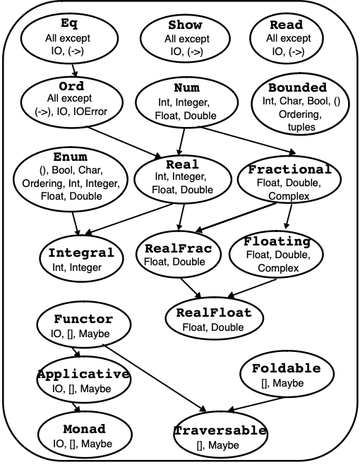{#ClassesDiagram width=“3.5in”}
Finally we have default definitions for the maximum and minimum operations,
max x y
| x <= y = y
| otherwise = x
min x y
| x <= y = x
| otherwise = y
Most Haskell types belong to these equality and ordering classes: among the exceptions are function types, and some of the abstract data types we meet below in Abstract data types.
It is useful to generate lists like [2,4,6,8] using the enumeration expression
[2,4 .. 8]
but enumerations can be built over other types as well: characters, floating-point numbers, and so on. The class definition is
class (Ord a) => Enum a where
succ, pred :: a -> a
toEnum :: Int -> a
fromEnum :: a -> Int
enumFrom :: a -> [a] -- [n .. ]
enumFromThen :: a -> a -> [a] -- [n,m .. ]
enumFromTo :: a -> a -> [a] -- [n .. m]
enumFromThenTo :: a -> a -> a -> [a] -- [n,n' .. m]
where enumFromTo and enumFromThenTo have default definitions, which we leave as exercises for the reader.
The signature of the class also contains operations fromEnum and toEnum which convert between the type and Int. Finally, the class contains succ and pred which step through the enumeration upwards and downwards: when succ is called at the greatest element, an error is returned.
Confusingly, the Haskell report states that ‘these functions [toEnum and fromEnum] are not meaningful for all instances of Enum’, and using these operations over floating-point values or full precision integers will result in a run-time error.
Full instances of the class include Int, Char, Bool and other finite types like Ordering.
and the two values give the minimum and maximum values in these types. The types Int, Char, Bool, Ordering belong to this class. Types that are in both Bounded and Enum obey some extra constraints that are explained in detail in the Haskell 2010 report (Marlow 2010).
The standard prelude defines the class Show, which contains types whose values can be written (or ‘shown’) as strings.
type ShowS = String -> String
class Show a where
showsPrec :: Int -> a -> ShowS
show :: a -> String
showList :: [a] -> ShowS
The function showsPrec supports flexible and efficient conversion of large data values, but in an introductory context, the function
show :: a -> String
which converts a value into a string is all that is needed. The class contains default definitions of showsPrec from show and vice versa. Further details about how to exploit the subtleties of showsPrec can be found in Hudak et al. (2000).
Most types belong to the class Show, but absent are function types and IO. For other types, example instance declarations might be
instance Show Bool where
show True = "True"
show False = "False"
instance (Show a, Show b) => Show (a,b) where
show (x,y) = "(" ++ show x ++ "," ++ show y ++ ")"
The class Read contains types whose values can be read from strings. To use the class it is enough to know about the function
read :: (Read a) => String -> a
The result of a read may not be properly defined: there needs to be exactly one object of the required type in the input string (which may optionally also contain whitespace or nested comments); in any other case the read will fail with an error. More details of how strings are parsed in this way can be found in Case study: parsing expressions.
It is also important to see that in many cases the type of the result of the read has to be specified, since it could potentially be of any type in the class Read. For instance, we can write
(read " 1 ") :: Int
which indicates that in this case we require the result of the read to be an Int. Without this type declaration we get this error on evaluating (read " 1 "):
Ambiguous type variable `a' in the constraint:
`Read a' arising from a use of `read' at <interactive>:1:0-8
Probable fix: add a type signature that fixes these type variable(s)
The class Read complements Show, since strings produced by show are usually readable by read. Many types can be read, but exclusions include function types.
One of the purposes of the Haskell design was to build a functional programming language which had a strong type system – in which any type errors in definitions and expressions are found before evaluation – yet which contains a rich set of numeric types, as befits a language suitable to substantial ‘real world’ tasks. Among Haskell’s numeric types are
The fixed precision integers, Int, and the full precision integers, Integer, which represent all integers faithfully.
The floating-point numbers, Float, and the double-precision floating-point numbers, Double.
Rational numbers, that is fractions, represented as ratios of integers; built-in is the type Rational of Integer fractions.
Complex numbers, which can be built over other types such as Float.
The design also required that the usual operations like + and / and literals such as 23 and 57.4 would be overloaded. For instance, Int and Integer will carry identical operations3 and have identical literals, as indeed will Float and Double; a guide to the operations over integers and floats was given in The integers: Integer and Int and Floating-point numbers: Float. This overloading can lead to situations where the type of an expression is undetermined; in such a case we can give an explicit type to an expression, thus:
(2+3)::Int
The Haskell report (Marlow 2010), Section 4.3.4, discusses a mechanism by which a default type can be given to numeric expressions. These default directives mean that whole numbers are taken to be Integer and others to be Double in the absence of any other type information. This can be seen in action in this snapshot of GHCi:
Overloading of numeric functions is achieved by defining a collection of classes. Full details of these can be found in the Haskell report (Marlow 2010), and in the standard prelude, Prelude.hs; a brief introduction follows here.
The base class to which all numeric types belong is Num, which has the signature
class (Eq a, Show a) => Num a where
(+), (-), (*) :: a -> a -> a
negate :: a -> a
abs, signum :: a -> a
fromInteger :: Integer -> a
x - y = x + negate y
This signature has the effect that all numeric types carry equality and show functions, together with addition, subtraction, multiplication and related operations. It is also possible to convert an Int or and Integer into a value of any numeric type.
Integer literals are of any numeric type, so that, for example
2 :: Num a => a
The integer types belong to the class Integral among whose signature functions are
quot, rem :: a -> a -> a
div, mod :: a -> a -> a
which give two variants of integer division, ‘quot‘ truncating towards zero, and ‘div‘ truncating below.
Numbers with fractional parts have a substantially richer class structure. Literals of this kind belong to every type in the Fractional class,
2.3 :: Fractional a => a
which extends Num with fractional division and reciprocal,
class (Num a) => Fractional a where
(/) :: a -> a -> a
recip :: a -> a
fromRational :: Rational -> a
recip x = 1 / x
The floating-point numbers in Float and Double belong to the class Floating, which carries the ‘mathematical’ functions. A part of its signature follows,
class (Fractional a) => Floating a where
pi :: a
exp, log, sqrt :: a -> a
(**), logBase :: a -> a -> a
sin, cos, tan :: a -> a
....
and the full signature is to be found in Prelude.hs. Further details of this and the complex and rational types can be found in the prelude, libraries and the Haskell documentation.
When a new data type is introduced, it comes with facilities for pattern matching but no other pre-defined functions. On the other hand, it’s possible to come up with standard definitions of equality, ordering, show and read functions for these types, and this deriving mechanism is the bit of ‘Haskell magic’ which we mentioned in Defining types for ourselves: enumerated types and Introducing algebraic types when we introduced data type definitions. If we make a definition like
data People = Person Name Age
deriving (Eq,Show)
then definitions of == and show which “do the obvious thing” are synthesised for this type. This could be done for all the standard classes, but we could also choose to define instances of other standard classes for ourselves, so that we might read name, age pairs from a comma separated variable (CSV) file, rather than using the standard definition of read, which would expect input of the form
13.10 Investigate the Haskell definition of ‘<’ on the types Bool and (t1,t2,…,tk).
13.11 Define a function
showBoolFun :: (Bool -> Bool) -> String
which displays a Boolean function as a table. Generalize this to
showBoolFunGen :: (a -> String) -> (Bool -> a) -> String
whose first argument is a function to show elements of a. This argument is used in giving a table of the results of the function. How would you extend your answer to deal with multiple-argument Boolean functions?
13.12 Using your answer to the previous question, or otherwise, describe how you would make Bool -> Bool an instance of the class Show. (Note, however, that this will not be legitimate Haskell 2010, since Bool -> Bool is not of the right form for an instance declaration; you can achieve this using the GHC option -XFlexibleInstances.)
13.13 How can you write a general instance for Show for function types: you could do this by showing a “sample” of the values from the function, that is showing how a sample of inputs are sent to the corresponding outputs.
13.14 Some types are not enumerated in the sense that they can be listed from smallest to largest: a good example is the Move type from the Rock - Paper - Scissors game. Define a type class to which the Move type can belong, and give an instance for Move. What other types can you think of giving an instance for: give some examples and their instances, too.
13.15 Define a data type Roman like this
data Roman = Roman Integer
and define instances of Show and Num for this type. The show function should display numbers in the form of Roman numerals, so that
show (Roman 99) = "IC"
show (Roman 1327) = "MCCCXXVII"
and so forth. The instance of Num should obey
(Roman n) + (Roman m) ~> Roman (n+m)
13.16 [Harder] For the data type Roman define an instances of the Read class, which is the inverse of the show function in the previous question.
Type classes and object-oriented programming
This note discusses the relationship between Haskell type classes and the classes of object-oriented programming; it can be omitted on first reading.
The type system of Haskell can be seen as giving monomorphic types to functions. Polymorphic types like
show :: Show a => a -> String
which involve type classes can be seen as shorthand for collections of typings, such as
show :: Bool -> String
show :: Char -> String
for each type Bool, Char, … belonging to the class.
In Haskell a class is a collection of types. Other languages such as C++ make a type and a class the same thing. Under that approach, introducing the class of visible objects would effectively give us a type4ShowType. This class would be characterized by having the function
show :: ShowType -> String
in its interface. The class ShowType would have Bool and Char among its sub-classes (or sub-types). This would allow us to write values like
[True,'N',False] :: [ShowType]
Moreover, to convert such a list to a String we could write
concat . map show :: [ShowType] -> String
At different items of the list we use different versions of the show function; on the first we use the Bool function, on the second the Char function and so forth. This so-called dynamic binding is a powerful feature of many object-oriented languages, including C++, but it is not a feature of Haskell 98; an extension which would allow dynamic binding is described in L"aufer (1996).
Returning to our example, what is the type of concat . map show in Haskell? It is not hard to see that it is
Show a => [a] -> [Char]
so that it can be applied to elements of [Bool], [Char] and so on, but not to heterogeneous lists like [True,’N’,False] which are not legitimately typed in Haskell.
Java allows users to define interfaces, which consist of a signature. A part of a class definition can say which interfaces the class implements. This is very like the way in which Haskell types are made instances of type classes, except that in Haskell it is not necessary to make the instance declaration a part of the type definition itself. This has the effect of allowing post hoc extensions to the operations supported by a type, in a way which is not possible for a class in Java.
Now that we have covered classes, we can see that every value in Haskell has a defined type, which might be monomorphic, polymorphic, or involve one or more type class constraints in a context. For example,
'w' :: Char
flip :: (a -> b -> c) -> (b -> a -> c)
elem :: Eq a => a -> [a] -> Bool
Strong typing means that we can check whether or not expressions we wish to evaluate or definitions we wish to use obey the typing rules of the language without any evaluation taking place. The benefit of this is obvious: we can catch a whole lot of errors before we run a program.
Haskell types can be inferred from expressions and definitions, and so it is possible never to write a type declaration. For example, we can write a definition like this
prodFun f g = \x -> (f x, g x)
either in a module or directly in GHCi, and then ask for its type in CHGi like this:
Because of this facility, some Haskellers never write a type declaration, but others, including the author, always do: why?
The type of an object is the most important single piece of documentation for the object, since it tells us how it can be used – what arguments need to be passed to it, and what type the result has – without us having to understand precisely how it is implemented.
We can use a type declaration to give a more specific type to a definition. This was the mechanism underlying the first part of the book, which turned polymorphic functions into monomorphic versions. To be clear, if we define prodFun like this
prodFun :: (Int -> Bool) -> (Int -> Char) -> Int -> (Bool,Char)
prodFun f g = \x -> (f x, g x)
then it will have this more specific type. It is not difficult to recover the most general type for the definition: just comment out the type declaration.
In writing a type declaration we are saying what type we think a function has. We may have not got this right, and the function is properly typed, but has a different type. For instance, typing
fun :: Int -> Bool -> Int
fun True 0 = 0
fun True n = n-1
fun _ n = n
gives rise to this error in GHCi:
Couldn't match expected type `Int' against inferred type `Bool'
In the pattern: True
In the definition of `fun': fun True 0 = 0
In a case like this it is useful to know that we were wrong, and then we can either correct the type declaration, or modify the function so that it has the type we wanted. Here the problem is fixed by swapping the types of the two arguments.
There is one case where we do need to use type declarations or annotations: this is in resolving ambiguity due to overloading (we talked briefly about this earlier, in The Haskell numeric types and classes).
Types are also useful in locating functions in a library. Suppose we want to define a function to remove the duplicate elements from a list, transforming [2,3,2,1,3,4] to [2,3,1,4], for instance. Such a function will have type
(Eq a) => [a] -> [a]
A Hoogle search of the standard prelude and libraries reveals just one function of this type, namely nub, which does exactly what we want. Plainly in practice there might be multiple matches (or missed matches because of the choice of parameter order) but nonetheless the types provide a valuable way into the Haskell library.
In the remainder this chapter we give an informal overview of the way in which types are checked. We start by looking at how type checking works in a monomorphic framework, in which every properly typed expression has a single type. Building on this, we then look at the polymorphic case, and see that it can be understood by looking at the constraints put on the type of an expression by the way that the expression is constructed. Crucial to this is the notion of unification, through which constraints are combined. We conclude the chapter by looking at the contexts which contain information about the class membership of type variables, and which thus manage overloading.
In this section we look at how type checking works in a monomorphic setting, without polymorphism or overloading. The main focus here is type-checking function applications. The simplified picture we see here prepares us for Haskell type checking in general, which is examined in the section after this.
We look first at the way that we type-check expressions, and then look at how definitions are type-checked.
In general, an expression is either a literal, a variable or a constant or it is built up by applying a function to some arguments, which are themselves expressions.
The case of function applications includes rather more than we might at first expect. For example, we can see list expressions like [True,False] as the result of applying the constructor function, ‘:’, thus: True:[False]. Also, operators and the if …then …else construct act in exactly the same way as functions, albeit with a different syntax.
The rule for type checking a function application is set out in the following diagram, where we see that a function of type s -> t must be applied to an argument of type s. A properly typed application results in an expression of type t.
We now look at two examples. First we take (not False) && True, a correctly typed expression of type Bool,
The application of not to False results in an expression of type Bool. The second argument to && is also a Bool, so the application of && is correctly typed, and gives a result of type Bool.
If we modify the example to (not ’c’) && True, we now see a type error, since a character argument, ’c’, is presented to an operator expecting a Bool argument, not.
The GHCi error message for this indicates the cause of the problem:
Couldn't match expected type `Bool' against inferred type `Char'
In the first argument of `not', namely 'c'
In the first argument of `(&&)', namely `(not 'c')'
In the expression: (not 'c') && True
In type-checking a monomorphic function definition such as
f :: t1 -> t2 -> ... -> tk -> t -- (fdef)
f p1 p2 ... pk
| g1 = e1
| g2 = e2
...
| gl = el
we need to check three things.
Each of the guards gi must be of type Bool.
The value ei returned in each clause must be of type t.
The pattern pj must be consistent with type of that argument, namely tj.
A pattern is consistent with a type if it will match (some) elements of the type. We now look at the various cases. A variable is consistent with any type; a literal is consistent with its type. A pattern (p:q) is consistent with the type [t] if p is consistent with t and q is consistent with [t]. For example, (0:xs) is consistent with the type [Int], and (x:xs) is consistent with any type of lists. The other cases of the definition are similar.
This concludes our discussion of type checking in the monomorphic case; we turn to polymorphism next.
Exercises
13.17 Predict the type errors you would obtain by defining the following functions
f n = 37+n
f True = 34
g 0 = 37
g n = True
h x
| x>0 = True
| otherwise = 37
k x = 34
k 0 = 35
Check your answers by typing each definition into a Haskell script, and loading the script into GHCi. Remember that you can use :type to give the type of an expression.
In a monomorphic situation, an expression is either well typed, and has a single type, or is not well typed and has none. In a polymorphic language like Haskell, the situation is more complicated, since a polymorphic object is precisely one which has many types.
In this section we first re-examine what is meant by polymorphism, before explaining type checking by means of constraint satisfaction. Central to this is the notion of unification, by which we find the types simultaneously satisfying two type constraints.
whose types are polymorphic, but how should we understand the type variable a in this type? We can see (length) as shorthand for saying that length has a set of types,
[Int] -> Int
[(Bool,Char)] -> Int
...
in fact containing all the types [t] -> Int where t is a monotype, that is a type not containing type variables.
When we apply length we need to determine at which of these types length is being used. For example, when we write
length ['c','d']
we can see that length is being applied to a list of Char, and so we are using length at type [Char] -> Int.
How can we explain what is going on here in general? We can see different parts of an expression as putting different constraints on its type. Under this interpretation, type checking becomes a matter of working out whether we can find types which meet the constraints. We have seen some informal examples of this when we discussed the types of map and filter in Higher-order functions: functions as arguments. We consider some further examples now.
The argument of f is a pair, and we consider separately what constraints there are on the types of x and y. x is completely unconstrained, as it is returned as the first half of a pair. On the other hand, y is used within the expression [’a’ .. y], which denotes a range within an enumerated type, starting at the character ’a’. This forces y to have the type Char, and gives the type for f:
What constraints are placed on the types of m and zs in this definition? We can see that m is added to something, so m must have a numeric type – which one it is remains to be seen. The other argument of the addition is length zs, which tells us two things.
First, we see that zs will have to be of type [b], and also that the result is an Int. This forces + to be used at Int, and so forces m to have type Int, giving the result
We now consider the composition of the last two examples,
h = g . f
In a composition g . f, the output of f becomes the input of g,
Here we should recall the meaning of types which involve type variables; we can see them as shorthand for sets of types. The output of f is described by (a,[Char]), and the input of g by (Int,[b]). We therefore have to look for types which meet both these descriptions. We will now look at this general topic, returning to the example in the course of this dicussion.
How are we to describe the types which meet the two descriptions (a,[Char]) and (Int,[b])?
As sets of types, we look for the intersection of the sets given by (a,[Char]) and (Int,[b]). How can we work out a description of this intersection? Before we do this, we revise and introduce some terminology.
Recall that an instance of a type is given by replacing a type variable or variables by type expressions. A type expression is a common instance of two type expressions if it is an instance of each expression. The most general common instance of two expressions is a common instance mgci with the property that every other common instance is an instance of mgci.
Now we can describe the intersection of the sets given by two type expressions. It is called the unification of the two, which is the most general common instance of the two type expressions.
Unification need not result in a monotype. In the example of unifying the types (a,[a]) and ([b],c),
the result is the type ([b],[[b]]). This is because the expression (a,[a]) constrains the type to have in its second component a list of elements of the first component type, while the expression ([b],c) constrains its first component to be a list. Thus satisfying the two gives the type ([b],[[b]]).
In the last example, note that there are many common instances of the two type expressions, including ([Bool],[[Bool]]) and ([[c]],[[[c]]]), but neither of these examples is the unifier, since ([b],[[b]]) is not an instance of either of them. On the other hand, they are each instances of ([b],[[b]]), as it is the most general common instance, and so the unifier of the two type expressions.
Not every pair of types can be unified: consider the case of [Int] -> [Int] and a -> [a].
Unifying the argument types requires a to become [Int], while unifying the result types requires a to become Int; clearly these constraints are inconsistent, and so the unification fails.
As we saw in Monomorphic type checking, function application is central to expression formation. This means that type checking also hinges on function applications.
In applying a function f :: s -> t to an argument e :: u we do not require that s and u are equal, but instead that they are unifiable to a type s’, say, giving e :: s’ and f :: s’ -> t’; the result in that case is of type t’.
As an example, consider the application map Circle where Circle is one of the constructor functions for the Shape type.
map :: (a -> b) -> [a] -> [b]
Circle :: Float -> Shape
Unifying a -> b and Float -> Shape results in a becoming Float and b becoming Shape; this gives
map :: (Float -> Shape) -> [Float] -> [Shape]
and so
map Circle :: [Float] -> [Shape]
As in the monomorphic case, we can use this discussion of typing and function application in explaining type checking all aspects of expressions. We now look at another example, before examining a more technical aspect of type checking.
foldr f s [] = s -- (foldr.1)
foldr f s (x:xs) = f x (foldr f s xs) -- (foldr.2)
which could be used to fold an operator into a list, as in
foldr (+) 0 [2,3,1] = 2+(3+(1+0))
so that it appears as if foldr has the type given by
foldr :: (a -> a -> a) -> a -> [a] -> a
In fact, the most general type of foldr is more general than this. Suppose that the starting value has type b and the elements of the list are of type a
foldr :: (... -> ... -> ...) -> b -> [a] -> ...
Then we can picture the definition thus:
s is the result of the first equation, and so the result type of the foldr function itself will be b, the type of s
foldr :: (... -> ... -> ...) -> b -> [a] -> b
In the second equation, f is applied to x as first argument, giving
foldr :: (a -> ... -> ...) -> b -> [a] -> b
The second argument of f is the result of a foldr, and so of type b,
foldr :: (a -> b -> ...) -> b -> [a] -> b
Finally, the result of the second equation is an application of f; this result must have the same result type as the foldr itself, b.
foldr :: (a -> b -> b) -> b -> [a] -> b
With this insight about the type of foldr we were able to see that foldr could be used to define another whole cohort of list functions, such as an insertion sort,
iSort :: Ord a => [a] -> [a]
iSort = foldr ins []
in which ins has the type Ord a => a -> [a] -> [a].
The first occurrence of [] is at [Bool], whilst the second is at [Integer]. This is completely legitimate, and is one of the advantages of a polymorphic definition. Now suppose that we replace the [] by a variable, and define
The variable xs is forced to have type [Bool]and type [Integer]; it is forced to be polymorphic, in other words. This is not allowed in Haskell, as there is no way of expressing the type of funny. It might be thought that
funny :: [a] -> Int
was a correct type, but this would mean that funny would have all the instance types
funny :: [Int] -> Int
funny :: [[Char]] -> Int
...
which it clearly does not. We conclude that constants and variables are treated differently: constants may very well appear at different incompatible types in the same expression, variables cannot.
What is the significance of disallowing the definition (funny) but allowing the definition (expr)? Taking (expr) first, we have a polymorphic definition of the form [] :: [a] and an expression in which [] occurs twice; the first occurrence is at [Bool], the second at [Integer]. To allow these independent uses to occur, we type-check each use of a polymorphic definition with different type variables, so that a constraint on one use does not affect any of the others.
On the other hand, how is the definition of (funny) disallowed? When we type check the use of a variable we will not treat each instance as being of an independent type. Suppose we begin with no constraint on xs, so xs::t, say. The first occurrence of xs forces xs::[Bool], the second requires xs::[Integer]; these two constraints cannot be satisfied simultaneously, and thus the definition (funny) fails to type check.
The crucial point to remember from this example is that the definition of a function can’t force any of its arguments to be polymorphic.
In type checking a function definition like (fdef) above we have to obey rules similar to the monomorphic case.
Each of the guards gi must be of type Bool.
The value ei returned in each clause must have a type si which is at least as general as t; that is, si must have t as an instance.
The pattern pj must be consistent with type of that argument, namely tj.
We take up a final aspect of type checking – the impact of type classes – in the next section.
Exercises
13.18 Do the following pairs of types – listed vertically – unify? If so, give a most general unifier for them; if not, explain why they fail to unify.
(Int -> b) (Int,a,a)
(a -> Bool) (a,a,[Bool])
13.19 Show that we can unify (a,[a]) with (b,c) to give (Bool,[Bool]).
13.20 Can the function
f :: (a,[a]) -> b
be applied to the arguments (2,[3]), (2,[]) and (2,[True]); if so, what are the types of the results? Explain your answers.
13.21 Repeat the previous question for the function
f :: (a,[a]) -> a
Explain your answers.
13.22 Give the type of f [] [] if f has type
f :: [a] -> [b] -> a -> b
What is the type of the function h given by the definition
h x = f x x ?
13.23 How can you use the Haskell system to check whether two type expressions are unifiable, and if so what is their unification? Hint: you can make dummy definitions in Haskell in which the defined value, zircon say, is equated with itself:
zircon = zircon
Values defined like this can be declared to have any type you wish.
13.24 [Harder] Recalling the definitions of curry and uncurry from Currying and uncurrying, what are the types of
curry id
uncurry id
curry (curry id)
uncurry (uncurry id)
uncurry curry
Explain why the following expressions do not type-check:
curry uncurry
curry curry
13.25 [Harder] Give an algorithm which decides whether two type expressions are unifiable. If they are, your algorithm should return a most general unifying substitution; if not, it should give some explanation of why the unification fails.
Classes in Haskell restrict the use of some functions, such as ==, to types in the class over which they are defined, in this case Eq. These restrictions are apparent in the contexts which appear in some types. For instance, if we define
member [] y = False
member (x:xs) y = (x==y) || member xs y
its type will be
Eq a => [a] -> a -> Bool
because x and y of type a are compared for equality in the definition, thus forcing the type a to belong to the equality class Eq.
This section explores the way in which type checking takes place when overloading is involved; the material is presented informally, by means of an example.
Suppose we are to apply the function member to an expression e, whose type is
Ord b => [[b]]
Informally, e is a list of lists of objects, which belong to a type which carries an ordering. In the absence of the contexts we would unify the type expressions, giving
member :: [[b]] -> [b] -> Bool e :: [[b]]
and so giving the application member e the type [b] -> Bool. We do the same here, but we also apply the unification to the contexts, producing the context
(Eq [b] , Ord b) -- (ctx.1)
Now, we check and simplify the context.
The requirements in a context can only apply to type variables, so we need to eliminate requirements like Eq [b]. The only way these can be eliminated is to use the instance declarations. In this case the built-in instance declaration
instance Eq a => Eq [a] where ....
allows us to replace the requirement Eq [b] with Eq b in (ctx.1), giving the new context
(Eq b , Ord b) -- (ctx.2)
We repeat this process until no more instances apply. If we fail to reduce all the requirements to ones involving a type variable, the application fails, and an error message would be generated. This happens if we apply member to [id];
No instance for (Eq (a -> a))
arising from a use of `member' at <interactive>:1:0-10
Possible fix: add an instance declaration for (Eq (a -> a))
In the expression: member [id]
In the definition of `it': it = member [id]
since id is a function, whose type is not it the class Eq.
We then simplify the context using the class definitions. In our example we have both Eq b and Ord b, but recall that
class Eq a => Ord a where ...
so that any instance of Ord is automatically an instance of Eq; this means that we can simplify (ctx.2) to
Ord b
This is repeated until no further simplifications result.
For our example, we thus have the type
member e :: Ord b => [b] -> Bool
This three-stage process of unification, checking (with instances) and simplification is the general pattern for type checking with contexts in Haskell.
Finally, we should explain how contexts are introduced into the types of the language. They originate in types for the functions in class declarations, so that, in the example of the Info class from earlier in the chapter, we have
examples :: Info a => [a]
size :: Info a => a -> Int
The type checking of functions which use these overloaded functions will propagate and combine the contexts as we have seen above.
We have seen informally how the Haskell type system accommodates type checking for the overloaded names which belong to type classes. A more thorough overview of the technical aspects of this, including a discussion of the ‘monomorphism restriction’ which needs to be placed on certain polymorphic bindings, is to be found in the Haskell 2010 report (Marlow 2010).
Exercises
13.26 Give the type of each of the individual conditional equations which follow, and discuss the type of the function which together they define.
This chapter has shown how names such as read and show and operators like + can be overloaded to have different definitions at different types. The mechanism which enables this is the system of Haskell classes. A class definition contains a signature which contains the names and types of operations which must be supplied if a type is to be a member of the class. For a particular type, the function definitions are contained in an instance declaration.
In giving the type of a function, or introducing a class or an instance, we can supply a context, which constrains the type variables occurring. Examples include
member :: Eq a => [a] -> a -> Bool
instance Eq a => Eq [a] where ....
class Eq a => Ord a where ....
In the examples, it can be seen that member can only be used over types in the class Eq. Lists of a can be given an equality, provided that a itself can; types in the class Ord must already be in the class Eq. After giving examples of the various mechanisms, we looked at the classes in the standard preludes of Haskell.
We concluded the chapter with a discussion of how type checking of expressions and definitions is performed in Haskell, initially in the monomorphic case, and then in full generality with polymorphic and overloaded functions. In that case we saw type checking as a process of extracting and consolidating constraints which come from the unification of type expressions which contain type variables.
In fact, the implementation of classes works like this, passing in a dictionary argument containing the appropriate equality function at each point that elem is used, after it has been transformed into elemGen. ↩
This gives a wide range of types to use in modelling different domains in Haskell. This chapter completes our coverage of the topic of algebraic types and looks at two extensions in some detail:
The types can be recursive; we can use the type we are defining, Typename, as (part of) any of the component types, as in the definition of numeric trees “NTrees”:
data NTree = NilT |
Node Integer NTree NTree
an illustration of a tree from NTree is given in An example of a tree of integers.. Recursion in data type definitions gives us lists, trees and many other useful data structures.
The name of the type being defined can be followed by one or more type variables which may be used on the right-hand side, making the definition polymorphic. An example built-into Haskell is the Maybe type,
data Maybe a = Nothing | Just a
which can be used in modelling program errors.
Recursive polymorphic types combine these two ideas, and this powerful mixture provides types which can be reused in many different situations – the built-in type of lists is an example which we have already seen. We’ll look again at the NTree and Maybe types later in this chapter, and other examples are given in the sections which follow.
Algebraic data type definitions are introduced by the keyword data, followed by the name of the type, an equals sign and then the constructors of the type being defined. The name of the type and the names of constructors begin with capital letters.
The general form of the algebraic type definitions which we have seen so far is
Each Coni is a constructor, followed by ki types, where ki is a non-negative integer which may be zero. We build elements of the type Typename by applying these constructor functions to arguments of the types given in the definition, so that
Coni vi1 ... viki
will be a member of the type Typename if vij is in tij for j ranging from 1 to ki. Reading the constructors as functions, the definition (Typename) gives the constructors the following types
Coni :: ti1 -> ... -> tiki -> Typename
Of the examples we have seen so far, enumerated types have constructors which take no arguments,
data Season = Spring | Summer | Autumn | Winter
product types have a single constructor,
data People = Person Name Age
and sum types are the most general: they have a number of constructors taking different arguments, as in the definition
data Shape = Circle Float |
Rectangle Float Float
Definitions over algebraic types use pattern matching both to distinguish between different alternatives and to extract components from particular elements:
area :: Shape -> Float
area (Circle r) = pi*r*r
area (Rectangle h w) = h*w
As we discussed in A tour of the built-in Haskell classes, Haskell has a number of built-in classes including Eq, Ord, Enum, Show, and Read. When we introduce a new algebraic type it’s possible to derive instances of these classes for the new type, like this:
data Season = Spring | Summer | Autumn | Winter
deriving (Eq,Ord,Enum,Show,Read)
We can thus compare seasons for equality and order, write expressions of the form [Spring .. Autumn] denoting the list [Spring, Summer, Autumn], and show and read values of the type.
Exercises
14.1 Reimplement the library database of A library database to use an algebraic type like People rather than a pair. Compare the two approaches to this example.
14.2 The library database of A library database is to be extended in the following ways.
CDs and videos as well as books are available for loan.
A record is kept of the authors of books as well as their titles. Similar information is kept about CDs, but not about videos.
Each loan has a period: books one month, CDs one week and videos three days.
Explain how you would modify the types used to implement the database, and how the function types might be changed. The system should perform the following operations. For each case, give the types and definitions of the functions involved.
Find all items on loan to a given person.
Find all books, CDs or videos on loan to a particular person.
Find all items in the database due back on or before a particular day, and the same information for any given person.
Update the database with loans; the constant today can be assumed to contain today’s date, in a format of your choice.
What other functions would have to be defined to make the system usable? Give their types, but not their definitions.
Types are often naturally described in terms of themselves. For instance, an integer expression is either a literal integer, like 347, or is given by combining two expressions using an arithmetic operator such as plus or minus, as in (3-1)+3.
data Expr = Lit Integer |
Add Expr Expr |
Sub Expr Expr
Similarly, a tree is either nil or is given by combining a value and two sub-trees. For example, the number 12 and the trees in Two trees. are assembled to give the tree in An example of a tree of integers..
Two trees.
As a Haskell type we say
data NTree = NilT |
Node Integer NTree NTree
Finally, we have already used the type of lists: a list is either empty ( []) or is built from a head and a tail – another list – using the list constructor ‘:’. Lists will provide a good guide to using recursive (and polymorphic) definitions. In particular they suggest how ‘general’ polymorphic higher-order functions over other algebraic types are defined, and how programs are verified. We now look at some examples in more detail.
The type Expr gives a model of the simple numerical expressions discussed above. These might be used in implementing a simple numerical calculator, for instance.
data Expr = Lit Integer |
Add Expr Expr |
Sub Expr Expr
Some examples are
2
Lit 2
2+3
Add (Lit 2) (Lit 3)
(3-1)+3
Add (Sub (Lit 3) (Lit 1)) (Lit 3)
where the informal expressions are listed in the left-hand column, and their Expr forms in the right. Given an expression, we might want to
evaluate it;
turn it into a string, which can then be printed;
estimate its size – count the operators, say.
Each of these functions will be defined in the same way, using primitive recursion. As the type is itself recursive, it is not a surprise that the functions which handle the type are also recursive. Also, the form of the recursive definitions follows the recursion in the type definition. For instance, to evaluate an operator expression we work out the values of the arguments and combine the results using the operator.
At the non-recursive, base cases – (Lit n) here – the value is given outright.
At the recursive cases, the values of the function at the sub-expressions from which the expression is formed – eval e1 and eval e2 here – can be used in calculating the result.
The show function has a similar form
show :: Expr -> String
show (Lit n) = show n
show (Add e1 e2)
= "(" ++ show e1 ++ "+" ++ show e2 ++ ")"
show (Sub e1 e2)
= "(" ++ show e1 ++ "-" ++ show e2 ++ ")"
as does the function to calculate the number of operators in an expression; we leave this as an exercise. Other exercises at the end of the section look at a different representation of expressions for which a separate type is used to represent the different possible operators. Next, we look at another recursive algebraic type, but after that we return to Expr and give an example of a non-primitive-recursive definition of a function to rearrange expressions in a particular way.
As another example, take the problem of finding out how many times a number, p say, occurs in a tree. The primitive recursion suggests two cases, depending upon the tree.
For a null tree, NilT, the answer must be zero.
For a non-null tree, (Node n t1 t2), we can find out how many times p occurs in the sub-trees t1 and t2 by two recursive calls; we have to make a case split depending on whether p occurs at the particular node, that is depending on whether or not p==n.
The final definition is
occurs :: NTree -> Integer -> Integer
occurs NilT p = 0
occurs (Node n t1 t2) p
| n==p = 1 + occurs t1 p + occurs t2 p
| otherwise = occurs t1 p + occurs t2 p
The exercises at the end of the section give a number of other examples of functions defined over trees using primitive recursion. We next look at a particular example where a different form of recursion is used.
The next example shows a definition which uses a more general recursion than we have seen so far. After showing why the generality is necessary, we argue that the function we have defined is total: it will give a result on all well-defined expressions.
The operation of addition over the integers is associative, so that the way in which an expression is bracketed is irrelevant to its value. We can, therefore, decide to bracket expressions involving ‘+’ in any way we choose. The aim here is to write a program to turn expressions into right bracketed form, as shown in Rearranging additions and in the following table:
which is primitive recursive: on the right-hand side of their definition the function try is only used on sub-expressions of the argument. This function will have the effect of transforming (AddL) to (AddR), but unfortunately (AddExL) will be sent to (AddExR):
((2+3)+4)+5 -- (AddExL)
(2+3)+(4+5) -- (AddExR)
Rearranging additions
The problem is that in transforming (AddL) to (AddR) we may produce another pattern we are looking for at the top level: this is precisely what happens when (AddExL) is transformed to (AddExR). We therefore have to call the function again on the result of the rearrangement
The equation (Add.2) will only be applied to the cases where (Add.1) does not apply – this is when e1 is either a Sub or a Lit expression. This is always the case in pattern matching; the first applicable equation is used.
When we use primitive recursion we can be sure that the recursion will terminate to give an answer: the recursive calls are only made on smaller expressions and so, after a finite number of calls to the function, a base case will be reached.
The assoc function is more complicated, and we need a more subtle argument to see that the function will always give a result. The equation (Add.1) is the tricky one, but intuitively, we can see that some progress has been made – some of the ‘weight’ of the tree has moved from left to right. In particular, one addition symbol has swapped sides. None of the other equations moves a plus in the other direction, so that after applying (Add.1) a finite number of times, there will be no more exposed addition symbols at the top level of the left-hand side. This means that the recursion cannot go on indefinitely, and so the function always leads to a result.
In Reasoning about algebraic types we’ll look at specifying QuickCheck properties for functions over algebraic types, including assoc, as well as showing how some of these can be proved by induction.
using the infix form of the constructor, given by surrounding it with back-quotes.
When an expression like this is shown, it appears in prefix form, so that the expression (Lit 3) ‘Add‘ (Lit 4) appears as
Add (Lit 3) (Lit 4)
In a data definition we can define Haskell operators which are themselves constructors. These constructors have the same syntax as operator symbols, except that their first character must be a ‘:’, which is reminiscent of ‘:’, itself an infix constructor. For our type of integer expressions, we might define
In describing one type, it is often useful to use others; these in turn may refer back to the original type: this gives a pair of mutually recursive types. A description of a person might include biographical details, which in turn might refer to other people. For instance:
data Person = Adult Name Address Bio |
Child Name
data Bio = Parent String [Person] |
NonParent String
In the case of a parent, the biography contains some text, as well as a list of their children, as elements of the type Person.
Suppose that we want to define a function which shows information about a person as a string. Showing this information will require us to show some biographical information, which itself contains further information about people. We thus have two mutually recursive functions:
showPerson (Adult nm ad bio)
= show nm ++ show ad ++ showBio bio
...
showBio (Parent st perList)
= st ++ concat (map showPerson perList)
...
which counts the number of operators in an expression.
14.5 Add the operations of multiplication and integer division to the type Expr, and redefine the functions eval, show and size to include these new cases. What does your definition of eval do when asked to perform a division by zero?
14.6 Instead of adding extra constructors to the Expr type, as in the previous question, it is possible to factor the definition thus:
data Expr = Lit Integer |
Op Ops Expr Expr
data Ops = Add | Sub | Mul | Div
Show how the functions eval, show and size are defined for this type, and discuss the changes you have to make to your definitions if you add the extra operation Mod for remainder on integer division.
14.8 Complete the redefinition of functions over Expr after it has been defined using the infix constructors :+: and :-:.
14.9 Define functions to return the left- and right-hand sub-trees of an NTree.
14.10 Define a function to decide whether a number is an element of an NTree.
14.11 Define functions to find the maximum and minimum values held in an NTree.
14.12 A tree is reflected by swapping left and right sub-trees, recursively. Define a function to reflect an NTree. What is the result of reflecting twice,reflect . reflect?
14.13 Define functions
collapse, sort :: NTree -> [Integer]
which turn a tree into a list. The function collapse should enumerate the left sub-tree, then the value at the node and finally the right sub-tree; sort should sort the elements in ascending order. For instance,
14.14 Complete the definitions of showPerson and showBio which were left incomplete in the text.
14.15 It is possible to extend the type Expr so that it contains conditional expressions, If b e1 e2, where e1 and e2 are expressions, and b is a Boolean expression, a member of the type BExp,
data Expr = Lit Integer |
Op Ops Expr Expr |
If BExp Expr Expr
The expression
If b e1 e2
has the value of e1 if b has the value True and otherwise it has the value of e2.
data BExp = BoolLit Bool |
And BExp BExp |
Not BExp |
Equal Expr Expr |
Greater Expr Expr
The five clauses here give
Boolean literals, BoolLit True and BoolLit False.
The conjunction of two expressions; it is True if both sub-expressions have the value True.
The negation of an expression. Not be has value True if be has the value False.
Equal e1 e2 is True when the two numerical expressions have equal values.
Greater e1 e2 is True when the numerical expression e1 has a larger value then e2.
Define the functions
eval :: Expr -> Integer
bEval :: BExp -> Bool
by mutual recursion, and extend the function show to show the redefined type of expressions.
Algebraic type definitions can contain the type variables a, b and so on, defining polymorphic types. The definitions are as before, with the type variables used in the definition appearing after the type name on the left-hand side of the definition. A simple example is
The built-in type of lists can be given by a definition like
infixr 5 :::
data List a = NilL | a ::: (List a)
deriving (Eq,Ord,Show,Read)
where the syntax [a], [] and ‘:’ is used for List a, NilList and :::. Note that we have given a fixity declaration for ::: to give it the same fixity and associativity as :, we can therefore write expressions like this:
Lists form a useful paradigm for recursive polymorphic types. In particular, we can see the possibility of defining useful families of functions over such types, and the way in which program verification can proceed by induction over the structure of a type.
The trees of Recursive algebraic types carry numbers at each node; there is nothing special about numbers, and we can equally well say that they have elements of an arbitrary type at the nodes:
data Tree a = Nil | Node a (Tree a) (Tree a)
deriving (Eq,Ord,Show,Read)
The definitions of depth and occurs carry over unchanged:
depth :: Tree a -> Integer
depth Nil = 0
depth (Node n t1 t2) = 1 + max (depth t1) (depth t2)
as do many of the functions defined in the exercises at the end of Recursive algebraic types. One of these is the function collapsing a tree into a list. This is done by visiting the elements of the tree ‘inorder’, that is visiting first the left sub-tree, then the node itself, then the right sub-tree, thus:
collapse :: Tree a -> [a]
collapse Nil = []
collapse (Node x t1 t2)
= collapse t1 ++ [x] ++ collapse t2
Type definitions can take more than one parameter. We saw earlier the example of the type whose elements were either a name or a number. In general we can form a type whose elements come either from a or from b:
data Either a b = Left a | Right b
deriving (Eq,Ord,Read,Show)
Members of the ‘union’ or ‘sum’ type are (Left x), with x::a, and (Right y) with y::b. The ‘name or number’ type is given by Either String Int and
Left "Duke of Prunes" :: Either String Int
Right 33312 :: Either String Int
We can tell whether an element is in the first half of the union by
isLeft :: Either a b -> Bool
isLeft (Left _) = True
isLeft (Right _) = False
To define a function from Either a b to Int, say, we have to deal with two cases,
fun :: Either a b -> Int
fun (Left x) = ... x ...
fun (Right y) = ... y ...
In the first case, the right-hand side takes x to an Int, so is given by a function from a to Int; in the second case y is taken to an Int, thus being given by a function from b to Int.
Guided by this, we can give a higher-order function which joins together two functions defined on a and b to a function on Either a b. The definition follows, and is illustrated in Joining together functions..
Joining together functions.
either :: (a -> c) -> (b -> c) -> Either a b -> c
either f g (Left x) = f x
either f g (Right y) = g y
If we have a function f::a -> c and we wish to apply it to an element of Either a b, there is a problem: what do we do if the element is in the right-hand side of the Either type? A simple answer is to raise an error
applyLeft :: (a -> c) -> Either a b -> c
applyLeft f (Left x) = f x
applyLeft f (Right _) = error "applyLeft applied to Right"
but in the next section we shall explore other ways of handling errors in more detail. Exercises
14.16 Investigate which of the functions over trees discussed in the exercises of Recursive algebraic types can be made polymorphic.
14.17 Define a function twist which swaps the order of a union
twist :: Either a b -> Either b a
What is the effect of (twist . twist)?
14.18 How would you define applyLeft using the function either?
14.19 Show that any function of type a -> b can be transformed into functions of type
a -> Either b c
a -> Either c b
14.20 How could you generalize either to join so that it has type
join :: (a -> c) -> (b -> d) -> Either a b -> Either c d
You might find the answer to the previous exercise useful here, if you want to define join using either.
The trees defined in the text are binary: each non-nil tree has exactly two sub-trees. We can instead define general trees with an arbitrary list of sub-trees, thus:
data GTree a = Leaf a | Gnode [GTree a]
The exercises which follow concern these trees.
Exercises
14.21 Define functions
to count the number of leaves in a GTree;
to find the depth of a GTree;
to sum a numeric GTree Int;
to find whether an element appears in a GTree;
to map a function over the elements at the leaves of a GTree; and
to flatten a GTree to a list.
In each case give the type of the function that you have defined.
14.22 How is the completely empty tree represented as a GTree?
How should a program deal with a situation which ought not to occur? Examples of such situations include
attempts to divide by zero, to take the square root of a negative number, and other arithmetical transgressions;
attempts to take the head of an empty list – this is a special case of a definition over an algebraic type from which one case (here the empty list) is absent.
This section examines the problem, giving three approaches of increasing sophistication. The simplest method is to stop computation and to report the source of the problem. This is indeed what the Haskell system does in the cases listed above, and we can do this in functions we define ourselves using the error function,
error :: String -> a
An attempt to evaluate the expression error "Circle with negative radius" in GHCi results in the message
*** Exception: Circle with negative radius
being printed and computation stopping.
The problem with this approach is that all the useful information in the computation is lost; instead of this, the error can be dealt with in some way without stopping computation completely. Two approaches suggest themselves, and we look at them in turn now.
Now, an attempt to take the tail of any list will succeed. In a similar way we could say
divide :: Integer -> Integer -> Integer
divide n m
| (m /= 0) = n `div` m
| otherwise = 0
so that division by zero gives some answer. For tl and divide there have been obvious choices about what the value in the ‘error’ case should be; for head there is not, and instead we can supply an extra parameter to head, which is to be used in the case of the list being empty.
hd :: a -> [a] -> a
hd y (x:_) = x
hd y [] = y
This approach is completely general; if a function f (of one argument, say) usually raises an error when cond is True, we can define a new function
fErr y x
| cond = y
| otherwise = f x
This approach works well in many cases; the only drawback is that we have no way of telling when an error has occurred, since we may get the result y from either the error or the ‘normal’ case. Alternatively we can use an error type to trap and process errors; this we look at now.
The previous approach works by returning a dummy value when an error has occurred. Why not instead return an error value as a result? We define the type
data Maybe a = Nothing | Just a
deriving (Eq,Ord,Read,Show)
which is effectively the type a with an extra value Nothing added. We can now define a division function errDiv thus
errDiv :: Integer -> Integer -> Maybe Integer
errDiv n m
| (m /= 0) = Just (n `div` m)
| otherwise = Nothing
and in the general case, where f gives an error when cond holds,
fErr x
| cond = Nothing
| otherwise = Just (f x)
The results of these functions are now not of the original output type, a say, but of type Maybe a. These Maybe types allow us to raise an error, potentially. We can do two things with a potential error which has been raised
we can transmit the error through a function, the effect of mapMaybe;
The function mapMaybe transmits an error value through the application of the function g. Suppose that g is a function of type a -> b, and that we are to lift it to operate on the type Maybe a. In the case of an argument Just x, g can be applied to the x to give a result, g x, of type b; this is put into Maybe b by applying the constructor function Just. On the other hand, if Nothing is the argument then Nothing is the result.
mapMaybe :: (a -> b) -> Maybe a -> Maybe b
mapMaybe g Nothing = Nothing
mapMaybe g (Just x) = Just (g x)
In trapping an error, we aim to return a result of type b, from an input of type Maybe a; we have two cases to deal with
in the Just case, we apply a function from a to b;
in the Nothing case, we have to give the value of type b which is to be returned. (This is rather like the value we supplied to hd earlier.)
The higher-order function which achieves this is maybe, whose arguments n and f are used in the Nothing and Just cases respectively.
Error-handling functions.
maybe :: b -> (a -> b) -> Maybe a -> b
maybe n f Nothing = n
maybe n f (Just x) = f x
We can see the functions mapMaybe and maybe in action in the examples which follow. In the first, a division by zero leads to a Nothing which passes through the lifting to be trapped – 56 is therefore returned:
The advantage of the approach discussed here is that we can first define the system without error handling, and afterwards add the error handling, using the mapMaybe and maybe functions together with the modified functions to raise the error. As we have seen numerous times already, separating a problem into two parts has made the solution of each, and therefore the whole, more accessible.
We revisit the Maybe type in Monads: languages for functional programming where we see that it is an example of a more general programming structure, a monad. In particular there we examine the relationship between the function mapMaybe and the map function over lists.
Exercises
14.23 Using the functions mapMaybe and maybe, or otherwise, define a function
process :: [Int] -> Int -> Int -> Int
so that process xs n m takes the nth and mth items of the list of numbers xs, and returns their sum. Your function should return 0 if either of the numbers is not one of the indices of the list: for a list of length p, the indices are 0, …, p-1 inclusive.
14.24 Discuss the advantages and disadvantages of the three approaches to error handling presented in this section.
14.25 What are the values of type Maybe (Maybe a)? Define a function
squashMaybe :: Maybe (Maybe a) -> Maybe a
which will ‘squash’ Just (Just x) to Just x and all other values to Nothing.
14.26 In a similar way to mapMaybe, define the function
composeMaybe :: (a -> Maybe b) ->
(b -> Maybe c) ->
(a -> Maybe c)
which composes two error-raising functions. How could you use mapMaybe, the function composition operator and the squash function to define composeMaybe?
14.27 The Maybe type could be generalized to allow messages to be carried in the Nothing part, thus:
data Err a = OK a | Error String
How do the definitions of mapMaybe, maybe and composeMaybe have to be modified to accommodate this new definition?
Algebraic data types provide us with a powerful mechanism for modelling types which occur both in problems themselves, and within the programs designed to solve them. In this section we suggest a three-stage method for finding the appropriate algebraic type definitions. We apply it in two examples: finding the ‘edit distance’ between two words, and a simulation problem.
An important moral of the discussion here is that we can start to design data types independently of the program itself. For a system of any size we should do this, as we will be more likely to succeed if we can think about separate parts of the system separately.
We shall have more to say about design of data types in the next two chapters.
In discussing the stages of design, we follow the example of finding the edit distance between two strings. This is the shortest sequence of simple editing operations which can take us from one string to the other.
The example is a version of a practical problem: in keeping a display (of windows or simple text) up-to-date, the speed with which updates can be done is crucial. It is therefore desirable to be able to make the updates from as few elementary operations as possible; this is what the edit distance program achieves in a different context.
We suppose that there are five basic editing operations on a string. We can change one character into another, copy a character without modifying it, delete or insert a character and delete (kill) to the end of the string. We also assume that each operation has the same cost, except a copy which is free.
To turn the string "fish" into "chips", we could kill the whole string, then insert the characters one-by-one, at a total cost of six. An optimal solution will copy as much of the string as possible, and is given by
inserting the character ’c’,
changing ’f’ to ’h’,
copying ’i’,
inserting ’p’,
copying ’s’, and finally
deleting the remainder of the string, "h".
In the remainder of this section we design a type to represent the editing steps, and after looking at another example of data type design, define a function to give an optimal sequence of editing steps from one string to another.
The analysis here can also be used to describe the difference between two lists of arbitrary type. If each item is a line of a file, the behaviour of the function is similar to the Unix diff utility, which is used to give the difference between two text files.
Now we look at the three stages of algebraic type definition in detail.
First we have to identify the types of data involved. In the example, we have to define
data Edit = ...
which represents the editing operations.
Next, we have to identify the different sorts of data in each of the types. Each sort of data is given by a constructor. In the example, we can change, copy, delete or insert a character and delete (kill) to the end of the string. Our type definition is therefore
The ‘...’ show that we have not yet said anything about the types of the constructors.
Finally, for each of the constructors, we need to decide what its components or arguments are. Some of the constructors – Copy, Delete and Kill – require no information; the others need to indicate the new character to be inserted, so
Suppose we want to model, or simulate, how the queues in a bank or Post Office behave; perhaps we want to decide how many bank clerks need to be working at particular times of the day. Our system will take as input the arrivals of customers, and give as output their departures. Each of these can be modelled using a type.
Inmess is the type of input messages. At a given time, there are two possibilities:
No-one arrives, represented by the 0-ary constructor No;
Someone arrives, represented by the constructor Yes. This will have components giving the arrival time of the customer, and the amount of time that will be needed to serve them.
Hence we have
data Inmess = No | Yes Arrival Service
type Arrival = Integer
type Service = Integer
Similarly, we have Outmess, the type of output messages. Either no-one leaves (None), or a person is discharged (Discharge). The relevant information they carry is the time they have waited, together with when they arrived and their service time. We therefore define
data Outmess = None | Discharge Arrival Wait Service
type Wait = Integer
In the general case, we have a choice: should we first use Copy, Delete, Insert or Change? If the first characters of the strings are equal we should copy; but if not, there is no obvious choice. We therefore try all possibilities and choose the best of them:
We can use to QuickCheck to test two of the fundamental properties of the transform function.
First, it should produce a list whose cost is no bigger than the cost of building up the target string letter by letter, and then killing the original string, a cost of length ys + 1: we can state this as the property
14.28 How would you modify the edit distance program to accommodate a Swap operation, which can be used to transform "abxyz" to "baxyz" in a single step?
14.29 Write a definition of the edit function described above, which when given a list of edits and a string st, returns the sequence of strings given by applying the edits to st in sequence.
14.30 Can you give other QuickCheck properties that you would expect the edit distance program to have? You could think, for example, about particular sorts of inputs, e.g. where the input is an initial segment of the output.
14.31 Give a calculation of transform "cat" "am". What do you conclude about the efficiency of the transform function?
14.32 [Harder] Can you give a more efficient implementation of the function calculating the transform?
The remaining questions are designed to make you think about how data types are designed. These questions are not intended to have a single ‘right’ answer, rather you should satisfy yourself that you have adequately represented the types which appear in your informal picture of the problem.
Exercises
14.33 It is decided to keep a record of vehicles which will use a particular car park. Design an algebraic data type to represent them.
14.34 If you knew that the records of vehicles were to be used for comparative tests of fuel efficiency, how would you modify your answer to the last question?
14.35 Discuss the data types you might use in a database of students’ marks for classes and the like. Explain the design of any algebraic data types that you use.
14.36 What data types might be used to represent the objects which can be drawn using an interactive drawing program? To give yourself more of a challenge, you might like to think about grouping of objects, multiple copies of objects, and scaling.
data Vector = Vec Float Float
class Movable a where
move :: Vector -> a -> a
reflectX :: a -> a
reflectY :: a -> a
rotate180 :: a -> a
rotate180 = reflectX . reflectY
data Point = Point Float Float
deriving Show
instance Movable Point where
move (Vec v1 v2) (Point c1 c2) = Point (c1+v1) (c2+v2)
reflectX (Point c1 c2) = Point c1 (-c2)
reflectY (Point c1 c2) = Point (-c1) c2
rotate180 (Point c1 c2) = Point (-c1) (-c2)
Movable objects (1).
data Figure = Line Point Point |
Circle Point Float
deriving Show
instance Movable Figure where
move v (Line p1 p2) = Line (move v p1) (move v p2)
move v (Circle p r) = Circle (move v p) r
reflectX (Line p1 p2) = Line (reflectX p1) (reflectX p2)
reflectX (Circle p r) = Circle (reflectX p) r
reflectY (Line p1 p2) = Line (reflectY p1) (reflectY p2)
reflectY (Circle p r) = Circle (reflectY p) r
instance Movable a => Movable [a] where
move v = map (move v)
reflectX = map reflectX
reflectY = map reflectY
Movable objects (2).
We start by building a class of types whose members are geometrical objects in two dimensions. The operations of the class are those to move the objects in various different ways.
We now work through the definitions, which are illustrated in Movable objects (1). and Movable objects (2).. Some moves will be dictated by vectors, so we first define
data Vector = Vec Float Float
The class definition itself is
class Movable a where
move :: Vector -> a -> a
reflectX :: a -> a
reflectY :: a -> a
rotate180 :: a -> a
rotate180 = reflectX . reflectY
and it shows the ways in which an object can be moved. First it can be moved by a vector, as in the diagram below.
data Name a = Pair a String
exam1 = Pair (Point 0.0 0.0) "Dweezil"
instance Named (Name a) where -- (1)
lookName (Pair obj nm) = nm
giveName nm (Pair obj _) = (Pair obj nm)
mapName :: (a -> b) -> Name a -> Name b
mapName f (Pair obj nm) = Pair (f obj) nm
instance Movable a => Movable (Name a) where -- (2)
move v = mapName (move v)
reflectX = mapName reflectX
reflectY = mapName reflectY
class (Movable b, Named b) => NamedMovable b -- (3)
instance Movable a => NamedMovable (Name a)
Named movable objects.
We can also reflect an object in the x-axis (the horizontal axis) or the y-axis (the vertical), or rotate a figure through 180° around the origin (the point where the axes meet). The default definition of rotate180 works by reflecting first in the y-axis and then the x, as we did with the Picture type in Introducing functional programming.
We can now define a hierarchy of movable objects; first we have the Point,
data Point = Point Float Float
deriving Show
To make Point an instance of Movable we have to give definitions of move, reflectX and reflectY over the Point type.
Here we can see that the move is achieved by adding the components v1 and v2 to the coordinates of the point. Reflection is given by changing the sign of one of the coordinates
reflectX (Point c1 c2) = Point c1 (-c2)
reflectY (Point c1 c2) = Point (-c1) c2
For this instance we override the default definition of rotate180 by changing the sign of both coordinates. This is a more efficient way of achieving the same transformation than the default definition.
rotate180 (Point c1 c2) = Point (-c1) (-c2)
Using the type of points we can build figures:
data Figure = Line Point Point |
Circle Point Float
and in the instance declaration of Movable for Figure given in Movable objects (2). we use the corresponding operations on Point; for example,
move v (Line p1 p2) = Line (move v p1) (move v p2)
move v (Circle p r) = Circle (move v p) r
This same approach works again when we consider a list of movable objects:
instance Movable a => Movable [a] where
move v = map (move v)
reflectX = map reflectX
and so on. Using overloading in this way has a number of advantages.
The code is much easier to read: at each point we write move, rather than movePoint, and so on.
We can reuse definitions; the instance declaration for Movable [a] makes lists of any sort of movable object movable themselves. This includes lists of points and lists of figures. Without overloading we would not be able to achieve this.
Many forms of data contain some sort of name, a String which identifies the object in question. What do we expect to be able to do with a value of such a type?
We should be able to identify the name of a value, and
we ought to be able to give a new name to a value.
These operations are embodied in the Named class:
class Named a where
lookName :: a -> String
giveName :: String -> a -> a
and an example of Named types is given by
data Name a = Pair a String
the one-constructor type whose two components are of type a and String. The instance declaration for this type is
instance Named (Name a) where -- (1)
lookName (Pair obj nm) = nm
giveName nm (Pair obj _) = (Pair obj nm)
An important aspect of object-oriented software development is the way in which one class can be built upon another, reusing the operations of the original class on the subclass. In this section we explore how to combine the Movable and Named classes, to give objects which are both movable and named. The section is rather more advanced, and can be omitted on first reading.
Suppose we are to add names to our movable objects – how might this be done? We examine one approach in the text, and another in the exercises.
Our approach is to build the type Name a where elements of type a are movable, that is Movable a holds. We then want to establish that the type Name a is in both the classes Movable and Named. We have shown the latter for any type a already in (1) above, so we concentrate on the former.
The crucial insight is that the naming is independent of the named type; any operation on the type can be lifted to work over named types thus:
mapName :: (a -> b) -> Name a -> Name b
mapName f (Pair obj nm) = Pair (f obj) nm
We can then argue that all the operations of the Movable class can be lifted.
instance Movable a => Movable (Name a) where -- (2)
move v = mapName (move v)
reflectX = mapName reflectX
reflectY = mapName reflectY
Now we already know that Named (Name a) by (1) above, so if we define a class combining these attributes
class (Movable b, Named b) => NamedMovable b -- (3)
we can declare the instance
instance Movable a => NamedMovable (Name a)
This last instance is established by showing that the two constraints of (3) hold when b is replaced by Name a, but this is exactly what (1) and (2) say given the constraint Movable a.
This completes the demonstration that NamedMovable (Name a) holds when we know that Movable a. It is worth realising that this demonstration is produced automatically by the Haskell system – we only need to type what is seen in Named movable objects..
This section has begun to illustrate how classes can be used in the software development process. In particular we have shown how our movable objects can be named in a way which allows reuse of all the code to move the objects.
Exercises
14.37 A different way of combining the classes Named and Movable is to establish the instance
instance (Movable b,Named c) => NamedMovable (b,c)
This is done by giving the instances
instance Movable b => Movable (b,c) where ....
instance Named c => Named (b,c) where ....
Complete these instance declarations.
14.38 Show that the method of the previous question can be used to combine instances of any two classes.
14.39 The example in the final part of this section shows how we can combine an arbitrary instance of the Movable class, a, with a particular instance of the Named class, String. Show how it can be used to combine an arbitrary instance of one class with a particular instance of another for any two classes whatever.
14.40 Extend the collection of operations for moving objects to include scaling and rotation by an arbitrary angle. This can be done by re-defining Movable or by defining a class MovablePlus over the class Movable. Which approach is preferable? Explain your answer.
14.41 Design a collection of classes to model bank accounts. These have different forms: current, deposit and so on, as well as different levels of functionality. Can you reuse the Named class here?
Verification for algebraic types follows the example of lists, as first discussed in Reasoning about programs. The general pattern of structural induction over an algebraic type states that the result has to be proved for each constructor; when a constructor is recursive, we are allowed to use the corresponding induction hypotheses in making the proof. We first give some representative examples in this section, and conclude with a rather more sophisticated proof.
To prove the property P(tr) for all finite tr of type Tree t we have to do two things.
Nil case
Prove P(Nil).
Node case
Prove P(Node x tr1 tr2) for all x of type t
assuming that P(tr1) and P(tr2) hold already.
The advice of Reasoning about programs about finding proofs can easily be carried over to the situation here. Now we give a representative example of a proof. We aim to prove for all finite trees tr that
map f (collapse tr) = collapse (mapTree f tr) -- (map-collapse)
which states that if we map a function over a tree, and then collapse the result we get the same result as collapsing before mapping over the list. The functions we use are defined as follows
map f [] = [] -- (map.1)
map f (x:xs) = f x : map f xs -- (map.2)
mapTree f Nil = Nil -- (mapTree.1)
mapTree f (Node x t1 t2)
= Node (f x) (mapTree f t1) (mapTree f t2) -- (mapTree.2)
collapse Nil = [] -- (collapse.1)
collapse (Node x t1 t2)
= collapse t1 ++ [x] ++ collapse t2 -- (collapse.2)
map f (collapse Nil)
= map f [] -- by (collapse.1)
= [] -- by (map.1)
collapse (mapTree f Nil)
= collapse Nil -- by (mapTree.1)
= [] -- by (collapse.1)
collapse (mapTree f (Node x tr1 tr2))
= collapse (Node (f x) (mapTree f tr1)
(mapTree f tr2)) -- by (mapTree.2)
= collapse (mapTree f tr1) ++ [f x] ++
collapse (mapTree f tr2) -- by (collapse.2)
and this finishes the proof in the Node case. As this is the second of the two cases, the proof is complete. ⬛
Structural induction for the type Maybe t becomes proof by cases – because the type is not recursive, in none of the cases is there an appeal to an induction hypothesis. The rule is
We have seen that not all functions are defined by primitive recursion. The example we saw in Recursive algebraic types was of the function assoc, which is used to rearrange arithmetic expressions represented by the type Expr. Recall that
with (assoc.1) being the non-primitive recursive case. We would like to prove that the rearrangement does not affect the value of the expression:
eval (assoc ex) = eval ex -- (eval-assoc)
for all finite expressions ex. The induction principle for the Expr type has three cases.
Lit case
Prove P(Lit n).
Add case
Prove P(Add e1 e2), assuming P(e1) and P(e2)
Sub case
Prove P(Sub e1 e2), assuming P(e1) and P(e2)
To prove (eval-assoc) for all finite expressions, we have the three cases given above. The Lit and Sub cases are given, respectively, by (assoc.4) and (assoc.3), but the Add case is more subtle. For this we will prove
by induction on the number of Adds which are left-nested at the top level of the expression e1 – recall that it was by counting these and noting that assoc preserves the total number of Adds overall that we proved the function would always terminate. Now, if there are no Adds at the top-level of e1, the equation (assoc.2) gives (eval-Add). Otherwise we rearrange thus:
eval (assoc (Add (Add f1 f2) e2)))
= eval (assoc (Add f1 (Add f2 e2))) -- by (assoc.1)
and since f1 contains fewer Adds at top level,
= eval (Add f1 (Add f2 e2))
= eval (Add (Add f1 f2) e2) -- by associativity of +
which gives the induction step, and therefore completes the proof. ⬛
This result shows that verification is possible for functions defined in a more general way than primitive recursion.
Checking properties in QuickCheck
Many of these properties can be checked in QuickCheck; we can define properties like this:
prop_assoc :: Expr -> Bool
prop_assoc expr =
eval expr == eval (assoc expr)
prop_depth :: NTree -> Bool
prop_depth t =
size t < 2^(depth t)
prop_collapse :: Eq b => (a -> b) -> Tree a -> Bool
prop_collapse f =
\t -> map f (collapse t) == collapse (mapTree f t)
To be checkable, we need to be able to generate random values of the types Expr, NTree and Tree a (for types a for which random values can be generated). We have done this in the module available online, and we will explain the code in more detail in Domain-Specific Languages.
where recall that (==Summer) is an operator section whose effect is to test whether its argument is equal to Summer.
14.43 Is it the case that the area of each Shape from Introducing algebraic types is non-negative? If so, give a proof; if not, give an example which shows that it is not the case.
14.46 Prove that the function twist has the property that
twist . twist = id
14.47 Explain the principle of structural induction for the type GTree. Formulate and prove the equivalent of the theorem relating map, mapTree and collapse for this type of trees.
Algebraic types sharpen our ability to model types in our programs: we have seen in this chapter how simple, finite types like Temp can be defined, as well as the more complex Either and recursive types. Many of these recursive types are varieties of tree: we looked at numerical trees; elements of the type Expr can also be thought of as trees representing the underlying structure of arithmetical expressions.
The type of lists gives a guiding example for various aspects of algebraic types.
The definition of the type is recursive and polymorphic, and many polymorphic higher-order functions can be defined over lists – this carries over to the various types of tree and the error type, Maybe, for example.
There is a simple principle for reasoning over lists, structural induction, which is the model for structural induction over algebraic types.
The chapter also gives guidelines for defining algebraic types. The definition can be given in three parts: first the type name is identified, then the constructors are named, and finally their component types are specified. As in other aspects of program development, this separation of concerns assists the system developer to produce simple and correct solutions.
Having introduced algebraic data types we are able to give more substantial examples of classes and their instances. We can see that the overloading that classes bring makes code both easier to read and more amenable to reuse; we can see in particular how software can be extended in a way that requires little modification to the code.
In the chapters to come, algebraic types will be an integral part of the systems we develop, and indeed in the next case study we exhibit various aspects of these types. We shall also explore a different approach to types: abstract data types, and see how this approach complements and contrasts with the use of algebraic data types.
When the type is not recursive, the induction principle gives a proof for all defined objects. An object of this type is defined if it is Nothing, or Just y for a defined y. ↩
We use the case study in this chapter as a vehicle to illustrate many of the features of the previous chapters – polymorphism, algebraic types and program design – and to illustrate the module system of Haskell, which is discussed first.
As we first saw in Modules, a module consists of a number of definitions of types, functions and so on, with a clearly defined interface stating what the module exports to other modules which use or import it. We also saw in Finding your way around the Haskell libraries that module names can be composite, as in Data.Bits, taking the form of hierarchical names.
Using modules to structure a large program has a number of advantages.
Parts of the system can be built separately from each other. Suppose we want to monitor traffic on a network: one module might produce the statistics, while another displays them in a suitable form. If we agree which statistics are to be presented (their type etc.), that is we agree the interface, then development of the two parts of the system can go on independently.
Parts of a system can be compiled separately; this is a great advantage for a system of any complexity.
Libraries of components can be reused, by importing the appropriate modules containing them.
In the definition of Haskell 2010, there is no identification between modules and files. Nonetheless, we choose here to write one module per file, and indeed this is required by GHC.
Now we look at the details of Haskell modules, before giving our case study which exhibits the system in action.
Each module is named, so an example named Ant might be
module Ant where
data Ants = ...
anteater x = ...
Note that the definitions all begin in the column under the keyword module; it is safest to make this the leftmost column of the file.
We also assume that a module Foo will live in the file Foo.hs; GHC allows module and file names to be different, but we recommend that you keep them the same.
The basic operation on modules is to import one into another, so in defining Bee we might say
module Bee where
import Ant
beeKeeper = ...
This means that the visible definitions from Ant can be used in Bee. By default the visible definitions in a module are those which appear in the module itself. If we define
module Cow where
import Bee
the definitions of Ants and anteater will not be visible in Cow. They can be made visible either by importing Ant explicitly, or by using the export controls discussed below to modify exactly what is exported from Bee.
since its only role is in defining the reverse function.
On the other hand, it might be too little: we perhaps want to export some of the definitions we imported from other modules. The modules Ant, Bee and Cow above provide an example of this.
We can control what is exported by following the name of the module with a list of what is to be exported. For instance, we say in the case of Bee
module Bee ( beeKeeper, Ants(..), anteater ) where ...
The list contains names of defined objects, such as beeKeeper, and also data types like Ants. In the latter case we follow the type name with (..) to indicate that the constructors of the type are exported with the type itself; if this is omitted, then the type acts like an abstract data type, which we investigate further in the next chapter. The (..) is not necessary for a type definition.
Such a list works on a definition-by-definition basis; we can also state that all the definitions in a module are to be exported, as in
module Bee ( beeKeeper, module Ant ) where ...
or equivalently
module Bee ( module Bee , module Ant ) where ...
where preceding the name of a module by the keyword module is shorthand for all the names defined within the module. The simple header
module Fish where
is therefore equivalent to
module Fish ( module Fish ) where
The Main module
Each system of modules should contain a top-level module called Main, which gives a definition to the name main. In a compiled system, this is the expression which is evaluated when the compiled code is run. In an interpreter like GHCi, where we can run code in any module, it is of less significance.
A module without a header is treated as though it contains the header
We can control how objects are to be imported, just as we can control their export. We do this by following the import statement with a list of objects, types or classes. For instance, if we choose not to import anteater from Ant we can write
import Ant ( Ants(..) )
stating that we want just the type Ants; we can alternatively say which names we wish to hide:
import Ant hiding ( anteater )
Suppose that in our module we have a definition of bear, and also there is an object named bear in the module Ant. How can we gain access to both definitions? The answer is that we use the qualified name Ant.bear for the imported object, reserving bear for the locally defined one.
A qualified name is built from the name of a module and the name of an object in that module, separated by a full stop. Note that there should be no white space between the ‘.’ and the two names, so as to avoid confusion with the composition operator. To use qualified names we should make the import like this:
import qualified Ant
In the qualified case we can also state which particular items are to be imported or hidden, just as in the unqualified case above. It is possible to use a local name for an imported module, as in
import Insect as Ant
which gives the local name Ant to the imported module Insect.
Qualified and unqualified names
When a file is imported unqualified, that is without the qualified keyword, it is still possible to used qualified naming, so after importing Ant we can use both anteater and Ant.anteater to name the anteater function defined in that module.
On the other hand, if a file is imported qualified then only qualified names can be used. This note also applies when a module is given a local name, as in
import qualified Ant as Insect
after which the anteater function can only be invoked using Insect.anteater.
One thing you need to be careful about is that you can’t use a qualified name for a function within the function definition itself, but only outside that definition.
The standard Prelude is implicitly imported into every module. If we wish we can modify this import, perhaps hiding one or more bindings thus
module Eagle where
import Prelude hiding (words)
so that we can give our own definition of the name words. If we import Eagle into another module, this module will also have explicitly to hide the import of words from the Prelude if conflicting definitions are to be avoided, and so we see that a re-definition of a Prelude function cannot be done ‘invisibly’, as it were.
If we also wish to have access to the original definition of words we can make a qualified import of the prelude,
import qualified Prelude
and use the original words by writing its qualified name Prelude.words.
Further information about the Haskell module system can be found in the language report (Marlow 2010); note that some of the details will be different in particular implementations.
Exercises
15.1 Can you get the effect of export controls using import? Can you get the effect of the qualifications of import using export controls? Discuss why both directives are included in the language.
15.2 Explain why you think it is the default that imported definitions are not themselves exported.
15.3 It is proposed to add the following option to the module export control and the import statement. If the item -module Dog appears, then none of the definitions in the module Dog is exported or imported. Discuss the advantages and disadvantages of this proposal. How would you achieve the effect of this feature in the existing Haskell module system?
Any computer system which is used seriously will be modified during its lifetime, either by the person or team who wrote it, or more likely by others. For this reason, all systems should be designed with change in mind.
We mentioned this earlier when we said that systems should be documented, with types given to all top-level definitions, and comments accompanying each script and substantial definition. Another useful form of description is to link each definition with proofs which concern it; if we know some of the logical properties of a function, we have a more solid conception of its purpose.
Documentation makes a script easier to understand, and therefore change, but we can give structure to a collection of definitions if they are split among modules or scripts, each script concerning a separate part of the overall system. The directives which link the files tell us how the parts of the system fit together. If we want to modify a particular part of a system, we should therefore be able to modify a single module (at least initially), rather than starting by modifying the whole of the system as a single unit.
How should we begin to design a system as a collection of modules? The pieces of advice which follow are aimed to make modification as straightforward as possible.
Each module should have a clearly identified role.
Each module should do one thing only. If a module has two separate purposes, these should be split between two separate modules. The chance of a change to one affecting the other is thereby reduced.
Each part of the system should be performed by one module: each module should do one thing completely; it should be self-contained, in other words. If performing one part of the whole is split between two modules, then either their code should be merged, or there should be a module defined with the single purpose of bringing the two components together.
Each module should export only what is necessary. It is then clearer what the effect of an import is: precisely the functions which are needed are imported. This process is often called information hiding in software engineering, which is itself the general study of principles for programming in the large.
Modules should be small. As a rule of thumb, no module should be larger than can be printed on two or three sides of paper.
We have also mentioned design for reuse, particularly in the context of polymorphic types and higher-order functions. The module will be the unit of reuse, and a library will be accessed by means of an import statement. Similar principles apply to the design of libraries. Each library should have a clearly defined purpose, like implementing a type together with basic operations over the type. In addition, we can say that
on including a general-purpose module, it is possible to suppress the definitions which are not used;
a qualified import can be used to avoid the name-clashes which can often occur: despite the (infinite) choice of names for functions, in practice we tend to choose from a very small subset!
The advice here might seem dry – what has been said is illustrated in the case study which follows. In the next chapter we will return to the idea of information hiding when we meet abstract data types. In the remainder of this chapter we examine the case study of Huffman coding, the foundations of which we explore now.
Electronic messages of various kinds are sent between machines and people by the billion each day. Such messages are usually sent as sequences of binary ‘bits’. For the transmission to be swift, the messages need to be coded as efficiently as possible. The area we explore here is how to build codes – translations of characters into sequences of bits – which produce messages as compact as possible.
Trees can be used to code and decode messages. Consider as an example the tree
We can see this as giving codes for the letters a, b and t by looking at the routes taken to reach the letters. For example, to get to b, we go right at the top node, and left at the next:
which gives b the code RL. Similarly, L codes a, and RR the letter t.
The codes given by trees are prefix codes; in these codes no code for a letter is the start (or prefix) of the code for another. This is because no route to a leaf of the tree can be the start of the route to another leaf. For more information about Huffman codes and a wealth of general material on algorithms, see Cormen et al. (1990).
A message is also decoded using the tree. Consider the message RLLRRRRLRR. To decode we follow the route through the tree given, moving right then left, to give the letter b,
where we have shown under each tree the sequence of bits remaining to be decoded. Continuing again from the top, we have the codes for a then t,
so the decoded message begins with the letters bat.
In full, the message is battat, and the coded message is ten bits long. The codes for individual characters are of different lengths; a is coded in one bit, and the other characters in two. Is this a wise choice of code in view of a message in which the letter t predominates? Using the tree
the coded message becomes RRRLLLRLL, a nine-bit coding. A Huffman code is built so that the most frequent letters have the shortest sequences of code bits, and the less frequent have more ‘expensive’ code sequences, justified by the rarity of their occurrence; Morse code is an example of a Huffman code in common use.
The remainder of the chapter explores the implementation of Huffman coding, illustrating the module system of Haskell. Exercises
15.4 What is the coding of the message battat using the following tree?
Compare the length of the coding with the others given earlier.
15.5 Using the first coding tree, decode the coded message RLLRLRLLRR. Which tree would you expect to give the best coding of the message? Check your answer by trying the three possibilities.
We now begin to implement the Huffman coding and decoding, in a series of Haskell modules. The overall structure of the system we develop is illustrated at the end of the chapter in The modules of the Huffman coding system..
As earlier, we first develop the types used in the system.
data Bit = L | R deriving (Eq,Show)
type HCode = [Bit]
and in the translation we will convert the Huffman tree to a table for ease of coding.
type Table = [ (Char,HCode) ]
The Huffman trees themselves carry characters at the leaves. We shall see presently that during their formation we also use information about the frequency with which each character appears; hence the inclusion of integers both at the leaves and at the internal nodes.
-- Types.hs
--
-- The types used in the Huffman coding example.
-- The interface to the module Types is written out
-- explicitly here, after the module name.
module Types ( Tree(Leaf,Node),
Bit(L,R),
HCode ,
Table ) where
-- Trees to represent the relative frequencies of characters
-- and therefore the Huffman codes.
data Tree = Leaf Char Int | Node Int Tree Tree
-- The types of bits, Huffman codes and tables of Huffman codes.
data Bit = L | R deriving (Eq,Show)
type HCode = [Bit]
type Table = [ (Char,HCode) ]
The file `Types.hs`.
The name of the file, with an indication of its purpose, is listed at the start of the file; each of the definitions is preceded by a comment as to its purpose.
Note that we have given a full description of what is exported by the module, by listing the items after the module name. For the data types which are exported, Tree and Bit, the constructors are exported explicitly; this could also be done by following their names with (..). This interface information could have been omitted, but we include it here as useful documentation of the interface to the module.
We have chosen to list the names imported here; the statement import Types would have the same effect, but would lose the extra documentation.
The purpose of the module is to define functions to code and decode messages: we export only these, and not the auxiliary function(s) which may be used in their definition. Our module therefore has the header
module Coding ( codeMessage , decodeMessage )
To code a message according to a table of codes, we look up each character in the table, and concatenate the results.
It is interesting to see that the function level definition here gives an exact implementation of the description which precedes it; using partial application and function composition has made the definition clearer.
We now define lookupTable, which is a standard function to look up the value corresponding to a ‘key’ in a table.
lookupTable :: Table -> Char -> HCode
lookupTable [] c = error "lookupTable"
lookupTable ((ch,n):tb) c
| ch==c = n
| otherwise = lookupTable tb c
Because it is not included in the list of identifiers in the module statement above, this definition is not exported.
To decode a message, which is a sequence of bits, that is an element of HCode, we use a Tree.
decodeMessage :: Tree -> HCode -> [Char]
We saw in Coding and decoding that decoding according to the tree tr has two main cases.
If we are at an internal Node, we choose the sub-tree dictated by the first bit of the code.
If at a leaf, we read off the character found, and then begin to decode the remainder of the code at the top of the tree tr.
When the code is exhausted, so is the decoded message.
decodeMessage tr
= decodeByt tr
where
decodeByt (Node n t1 t2) (L:rest)
= decodeByt t1 rest
decodeByt (Node n t1 t2) (R:rest)
= decodeByt t2 rest
decodeByt (Leaf c n) rest
= c : decodeByt tr rest
decodeByt t [] = []
The locally defined function is called decodeByt because it decodes ‘by t’.
The first coding tree and example message of Coding and decoding can be given by
Given a text, such as "battat", how do we find the tree giving the optimal code for the text? We explain it in a number of stages following Section 17.3 of Cormen et al. (1990).
We first find the frequencies of the individual letters, in this case giving
[('b',1),('a',2),('t',3)]
The main idea of the translation is to build the tree by taking the two characters occurring least frequently, and making a single character (or tree) of them. This process is repeated until a single tree results; the steps which follow give this process in more detail.
Each of (’b’,1), … is turned into a tree, giving the list of trees
[ Leaf 'b' 1 , Leaf 'a' 2 , Leaf 't' 3 ]
which is sorted into frequency order.
We then begin to amalgamate together trees: we take the two trees of lowest frequency, put them together, and insert the result in the appropriate place to preserve the frequency order.
[ Node 3 (Leaf 'b' 1) (Leaf 'a' 2) , Leaf 't' 3 ]
This process is repeated, until a single tree results
Implementing the system will involve us in designing various modules to perform the stages given above. We start by deciding what the modules will be and the functions that they will implement. This is the equivalent at the larger scale of divide and conquer; we separate the problem into manageable portions, which can be solved separately, and which are put together using the import and module statements. We design these interfacesbefore implementing the functions.
The three stages of conversion are summarized in Module directives for Huffman tree formation., which shows the module directives of the three component files. We have added as comments the types of objects to be exported, so that these directives contain enough information for the exported functions in the files to be used without knowing how they are defined.
Frequency.hs:
module Frequency ( frequency ) -- [Char] -> [(Char,Int)]
MakeTree.hs:
module MakeTree ( makeTree ) -- [(Char,Int)] -> Tree
import Types
CodeTable.hs:
module CodeTable ( codeTable ) -- Tree -> Table
import Types
Module directives for Huffman tree formation.
In fact the component functions frequency and makeTree will never be used separately, and so we compose them in the module MakeCode.hs when bringing the three files together. This is given in The module MakeCode.hs..
--
-- MakeCode.hs
--
-- Huffman coding in Haskell.
--
module MakeCode ( codes, codeTable ) where
import Types
import Frequency ( frequency )
import MakeTree ( makeTree )
import CodeTable ( codeTable )
-- Putting together frequency calculation and tree conversion
codes :: [Char] -> Tree
codes = makeTree . frequency
The module `MakeCode.hs`.
Our next task is to implement each module in full and we turn to that now.
The aim of the function frequency is to take a text such as "battat" to a list of characters, in increasing frequency of occurrence, [(’b’,1),(’a’,2),(’t’,3)]. We do this in three stages:
First we pair each character with the count of 1, giving
[('b',1),('a',1),('t',1),('t',1),('a',1),('t',1)]
Next, we sort the list on the characters, bringing together the counts of equal characters.
[('a',2),('b',1),('t',3)]
Finally, we sort the list into increasing frequency order, to give the list above.
The function uses two different sorts – one on character, one on frequency – to achieve its result. Is there any way we can define a single sorting function to perform both sorts?
We can give a general merge sort function, which works by merging, in order, the results of sorting the front and rear halves of the list.
mergeSort :: ([a]->[a]->[a]) -> [a] -> [a]
mergeSort merge xs
| length xs < 2 = xs
| otherwise
= merge (mergeSort merge first)
(mergeSort merge second)
where
first = take half xs
second = drop half xs
half = (length xs) `div` 2
The first argument to mergeSort is the merging function, which takes two sorted lists and merges their contents in order. It is by making this operation a parameter that the mergeSort function becomes reusable.
In sorting the characters, we amalgamate entries for the same character
The function toTreeList converts each character-number pair into a tree, thus
toTreeList = map (uncurry Leaf)
where note that we use the prelude function uncurry to make an uncurried version of the constructor function Leaf.
The function makeCodes amalgamates trees successively into a single tree
makeCodes [t] = t
makeCodes ts = makeCodes (amalgamate ts)
How are trees amalgamated? We have to pair together the first two trees in the list (since the list is kept in ascending order of frequency) and then insert the result in the list preserving the frequency order. Working top-down, we have
amalgamate :: [ Tree ] -> [ Tree ]
amalgamate (t1:t2:ts) = insTree (pair t1 t2) ts
When we pair two trees, we need to combine their frequency counts, so
pair :: Tree -> Tree -> Tree
pair t1 t2 = Node (v1+v2) t1 t2
where
v1 = value t1
v2 = value t2
where the value of a tree is given by
value :: Tree -> Int
value (Leaf _ n) = n
value (Node n _ _) = n
The definition of insTree, which is similar to that used in an insertion sort, is left as an exercise. Again, the definition of the exported function uses various others whose definitions are not visible to the ‘outside world’.
Here we give the function codeTable which takes a Huffman tree into a code table. In converting the tree Node n t1 t2 we have to convert t1, adding L at the front of the code, and t2 with R at the head. We therefore write the more general conversion function
convert :: HCode -> Tree -> Table
whose first argument is the ‘path so far’ into the tree. The definition is
convert cd (Leaf c n)
= [(c,cd)]
convert cd (Node n t1 t2)
= (convert (cd++[L]) t1) ++ (convert (cd++[R]) t2)
The codeTable function is given by starting the conversion with an empty code string
-- The main module of the Huffman example
module Main (main, codeMessage, decodeMessage, codes, codeTable ) where
import Types ( Tree(Leaf,Node), Bit(L,R), HCode , Table )
import Coding ( codeMessage, decodeMessage )
import MakeCode ( codes, codeTable )
-- Main expression: print the coded and decoded
-- example text "there is a green hill".
main = print decoded
-- The example message to be coded.
message :: String
message = "there are green hills here"
-- The Huffman tree generated from the example.
treeEx :: Tree
treeEx = codes "there is a green hill"
-- The coding table generated from the example.
tableEx :: Table
tableEx = codeTable (codes "there is a green hill")
-- The example in code.
coded :: HCode
coded = codeMessage tableEx message
-- The example coded and then decoded.
decoded :: String
decoded = decodeMessage treeEx coded
In this file we can include representative examples, using the major functions listed in the import statements; the code is illustrated in The Main module of the Huffman coding system..
The structure of the system is given in The modules of the Huffman coding system.. Modules are represented by boxes, and an arrow from A to B indicates that A.hs is imported into B.hs. An arrow is marked to indicate the functions exported by the included module, so that, for example, codes and codeTable are exported from MakeCode.hs to Main.hs.
If this coding system were to be used as a component of a larger system, a module directive could be used to control which of the four functions and the types are exported, after the module had been renamed. It is important to realize that the types will need to be exported (or be included in the file including Main.hs) if the functions are to be used.
We can write a top-level test for a system like this, by taking an example string, coding it and then decoding it. This should take us back to the string we started with, and indeed we can see this in the particular example in The Main module of the Huffman coding system.. It is possible to change this to a QuickCheck property, which checks that coding/decoding is the identity for a whole collection of strings; we leave this as an exercise for the reader.
The top-level test corresponds to a system test, in that it uses all the functions defined – implicitly or explicitly – and checks the overall functionality of the system. It is also possible to write unit tests, which check that a particular function or module has the required functionality.
For example, we might look at the module Frequency.hs, and in particular at the functions designed to merge or sort their arguments. A QuickCheck property embodying a unit test for these would include
where sorted expresses that its argument is sorted into ascending order and merge will merge two ordered lists in order.
Exercises
15.8 Give a definition of merge sort which uses the built-in ordering ‘<=’. What is its type?
15.9 Modifying your previous answer if necessary, give a version of merge sort which removes duplicate entries.
15.10 Give a version of merge sort which takes an ordering function as a parameter:
ordering :: a -> a -> Ordering
Explain how to implement mergeSort freqMerge using this version of merge sort, and discuss why you cannot implement mergeSort alphaMerge this way.
15.11 Define the insTree function, used in the definition of makeTree.
15.12 Give a calculation of
makeTree [('b',2),('a',2),('t',3),('e',4)]
15.13 Define functions
showTree :: Tree -> String
showTable :: Table -> String
which give printable versions of Huffman trees and code tables. One general way of printing trees is to use indentation to indicate the structure. Schematically, this looks like
left sub tree, indented by 4 characters
value(s) at Node
right sub tree, indented by 4 characters
15.14 Define a QuickCheck property to test coding and decoding: specifically this should code a string and decode it, and compare the result with the original. You may need to restrict the strings over which the test is made.
15.15 Define sorted so that it checks whether its argument is sorted into ascending order and define merge which will merge two ordered lists in order. Using these check whether the property prop_mergeSort :: [Int] -> Bool, defined earlier, holds.
15.16 Write QuickCheck unit tests for other functions in Frequency.hs and other modules of the Hufmann coding system.
15.17 You may find that it is necessary to restrict the domain over which some properties hold in order for them to QuickCheck successfully: can you re-define the functions involved so that the properties hold for all randomly generated inputs.
15.18 The correctness property for the Huffman system formulated earlier states that decode.code is the identity. Would you expect that code.decode is the identity: if so, over what domain; if not, can you give a sub-domain over which you wold expect it to hold?
When writing a program of any size, we need to divide up the work in a sensible way. The Haskell module system allows one script to be included in another. At the boundary, it is possible to control exactly which definitions are exported from one module and imported into another.
We gave a number of guidelines for the design of a program into its constituent modules. The most important advice is to make each module perform one clearly defined task, and for only as much information as is needed to be exported – the principle of information hiding. This principle is extended in the next chapter when we examine abstract data types.
The design principles were put into practice in the Huffman coding example. In particular, it was shown for the file MakeCode.hs and its three sub-modules that design can begin with the design of modules and their interfaces – that is the definitions (and their types) which are exported. Thus the design process starts before any implementation takes place.
The Haskell module system allows definitions of functions and other objects to be hidden when one module is imported into another. Those definitions hidden are only of use in defining the exported functions, and hiding them makes clearer the exact interface between the two modules: only those features of the module which are needed will be visible.
This chapter shows that information hiding is equally applicable for types, giving what are known as abstract data types, or ADTs. We explain the abstract data type mechanism here, as well as providing a number of examples of ADTs, including queues, sets, relations and the fundamental types belonging to a simulation case study.
We begin our discussion with a scenario which is intended to show both the purpose and the operation of the abstract data type mechanism.
Suppose we are to build a calculator for numerical expressions, like those given by the Expr type of Recursive algebraic types, but with variables included. The calculator is to provide the facility to set the values of variables, as well as for variables to form parts of expressions.
As a part of our system, we need to be able to model the current values of the variables, which we might call the store of the calculator. How can this be done? A number of models present themselves, including:
a list of integer/variable pairs: [(Integer,Var)]; and
a function from variables to integers: (Var -> Integer).
Both models allow us to look up and update the values of variables, as well as set a starting value for the store. These operations have types as follows.
initial :: Store
value :: Store -> Var -> Integer -- (StoreSig)
update :: Store -> Var -> Integer -> Store
but each model allows more than that: we can, for instance, reverse a list, or compose a function with others. In using the type Store we intend only to use the three operations given, but it is always possible to use the model in unintended ways.
How can we give a better model of a store? The answer is to define a type which only has the operations initial, value and update, so that we cannot abuse the representation. We therefore hide the information about how the type is actually implemented, and only allow the operations (StoreSig) to manipulate objects of the type.
When we provide a limited interface to a type by means of a specified set of operations we call the type an abstract data type (or ADT). Since the ‘concrete’ type itself is no longer accessible and we may only access the type by means of the operations provided, these operations give a more ‘abstract’ view of the type.
The Store abstract data type.
The Store abstract data type. illustrates the situation, and suggests that as well as giving a natural representation of the type of stores, there are two other benefits of type abstraction.
The type declarations in (StoreSig) form a clearly defined interface, which is called the signature of the ADT, between the user of the type and its implementer. The only information that they have to agree on is the signature; once this is agreed, they can work independently. This is therefore another way of breaking a complex problem into simpler parts; another aspect of the ‘divide and conquer’ method.
We can modifythe implementation of the Store without having any effect on the user. Contrast this with the situation where the implementation is visible to the user. In particular, if the implementation is an algebraic type then any change in the implementation will mean that all definitions that use pattern matching will have to be changed. These will include not just those in the signature, but also any user-defined functions which use pattern matching.
We shall see both aspects illustrated in the sections to come; first we look at the details of the Haskell abstract data type mechanism.
When we introduced the Haskell module system in Case study: Huffman codes we saw that there were two ways in which we could export a data type, called Data say. If we include Data(..) in the export list of the module, the type is exported with its constructors; if we include Data then the constructors are not exported, and so we can only operate over the type using the other operations of the signature.
In the case of the Store type, our module header would be
module Store ( Store, initial, value, update ) where
which shows that we can access the type only through the three functions mentioned. In this book we will adopt the convention that we will also include as comments in the module header the types of the exported functions, giving in the case of Store the following header.
module Store
( Store,
initial, -- Store
value, -- Store -> Var -> Integer
update -- Store -> Var -> Integer -> Store
) where
Now, the module must contain a definition of the Store type and the functions over it.
If the implementation type was a data type, then this would complete the realization of the abstract data type. However, in our running example of stores, we suggested earlier that we would use a list of pairs, [ (Integer,Var) ], to model the type, and so we will have to define a new data type, called Store
data Store = Store [ (Integer,Var) ]
which has a single constructor which we also call Store. This is the function which converts a list into an element of the Store type; we can think of it as ‘wrapping up’ a list to make it into a Store.
We now have to define the functions initial, value and update over the Store type. One approach is to define the analogous functions over [(Integer,Var)] and then to adapt those. We can say
init :: [(Integer,Var)]
init = []
val :: [(Integer,Var)] -> Var -> Integer
val [] v = 0
val ((n,w):sto) v
| v==w = n
| otherwise = val sto v
upd :: [(Integer,Var)] -> Var -> Integer -> [(Integer,Var)]
upd sto v n = (n,v):sto
The initial store, init, is represented by an empty list; the value of v is looked up by finding the first pair (n,v) in the list, and the store is updated by adding a new (Integer,Var) at the front of the list.
These functions then have to be converted to work over the type Store, so that arguments and results are of the form Store xs with xs::[(Integer,Var)]. The definitions become
initial :: Store
initial = Store []
value :: Store -> Var -> Integer
value (Store []) v = 0
value (Store ((n,w):sto)) v
| v==w = n
| otherwise = value (Store sto) v
update :: Store -> Var -> Integer -> Store
update (Store sto) v n = Store ((n,v):sto)
where we can see that the pattern of the definitions is similar, except that we have to ‘unwrap’ arguments of the form (Store sto) on the left-hand side, and ‘wrap up’ results using Store on the right-hand side. We look at a general mechanism for ‘wrapping up’ functions in the example of the Set ADT in Sets.
What happens if we try to break the abstraction barrier and deal with a Store as having the form (Store xs)? On typing
initial == Store []
in a module importing Store we get the type error message
Not in scope: data constructor `Store'
The fact that initial is indeed implemented as Store [] is irrelevant, since the implementation is not in scope outside the Store module.
In fact in this case rather than using a data type we will define
newtype Store = Store [ (Integer,Var) ]
which has the same effect as declaring a data type with one unary constructor but which is implemented in a more efficient fashion.
Naming newtypes
Another possible way of implementing the type would be to say
newtype Store = Sto [ (Integer,Var) ]
using different names for the type and its constructor. Although this makes it clear whether we are talking about the type or the constructor, we prefer to use a single name within this newtype, as otherwise we need to choose two different – but related – names.
Moreover, in practice, when we use Store we will always be able to tell which use – type name or constructor – is meant. Finally, this convention is in widespread use in the Haskell developer community, and so it’s helpful to be aware of the fact.
We can declare types as belonging to particular type classes such as Show and Eq, and this applies equally well to abstract data types. In the case of Store we can say
instance Eq Store where
(Store sto1) == (Store sto2) = (sto1 == sto2)
instance Show Store where
showsPrec n (Store sto) = showsPrec n sto
Note, however, that once declared, these instances cannot be hidden, so that even though they are not named in the export list, the functions over Store which are defined by means of these instance declarations will be available whenever the module Store is imported. Of course, we can choose not to declare these instances, and so not to provide an equality or a show function over Stores.
A different implementation of Store is given by the type of functions from variables to integers.
newtype Store = Store (Var -> Integer)
initial :: Store
initial = Store (\v -> 0)
value :: Store -> Var -> Integer
value (Store sto) v = sto v
update :: Store -> Var -> Integer -> Store
update (Store sto) v n
= Store (\w -> if v==w then n else sto w)
Under this implementation,
the initial store maps every variable to 0;
to look up a value of a variable v the store function sto is applied to v, and
in the case of an update, a function returned is identical to sto except on the variable whose value is changed.
Suppose that we have implemented a store as a list of integer-variable pairs. We can inspect the result of updating a store, which will be a new list, and check that it has the properties that we would expect. For example, we might take the difference of the lists before and after the update.
If we implement queues as an ADT, we can’t look directly at the underlying implementation; instead we have to write properties using the interface functions, here initial, value and update. We can start by saying what happens if we look up a value in the initial store:
What can we say about the effect of an update on a store? First, if perform an update for the variable ch and then look up the value, we would expect to see the new value:
prop_Update1 :: Char -> Integer -> Store -> Bool
prop_Update1 ch int st =
value (update st ch int) ch == int
Finally, what if we look up the value of another variable after this update? Its value should be the same as it was before:
prop_Update2 :: Char -> Char -> Integer -> Store -> Bool
prop_Update2 ch1 ch2 int st =
value (update st ch2 int) ch1 == value st ch1
If we perform a QuickCheck on these properties – the appropriate QuickCheck magic is given in the module StoreTest and the properties in QCStoreTest – the first two pass every time, but the third one sometimes fails: that is when ch1 and ch2 are equal!
Modifying the test to take this into account, we get a test that always passes:
prop_Update2 :: Char -> Char -> Integer -> Store -> Bool
prop_Update2 ch1 ch2 int st =
value (update st ch2 int) ch1 == value st ch1 || ch1==ch2
Because the tests are written in terms of the interface only, if we were to change the implementation then the tests could still be applied, assuming that we have the right QuickCheck definitions in place.
Exercises
16.1 Give an implementation of Store using lists whose entries are ordered according to the variable names. Discuss why this might be preferable to the original list implementation, and also its disadvantages, if any.
16.2 For the implementation of Store as a list type [(Integer,Var)], give a definition of equality which equates any two stores which give the same values to each variable. Can this operation be defined for the second implementation? If not, give a modification of the implementation which allows it to be defined.
16.3 In this question you should use the type Maybe a. Suppose it is an error to look up the value of a variable which does not have a value in the given store. Explain how you would modify both the signature of Store and the two implementations.
16.4 Rather than giving an error when looking up a variable which does not have a value in the particular store, extend the signature to provide a test of whether a variable has a value in a given store, and explain how would modify the two implementations to define the test.
16.5 Suppose you are to implement a fourth operation over Store
setAll :: Integer -> Store
so that setAll n is the store where every variable has the value n. Can you do this for both the example implementations? Show how if you can, and explain why, if not.
A queue is a ‘first in, first out’ structure. If first Flo and then Eddie joins an initially empty queue, the first person to leave will be Flo. As an abstract data type, we expect to be able to add items and remove items as well as there being an empty queue.
module Queue
( Queue ,
emptyQ , -- Queue a
isEmptyQ , -- Queue a -> Bool
addQ , -- a -> Queue a -> Queue a
remQ -- Queue a -> ( a , Queue a )
) where
The function remQ returns a pair – the item removed together with the part of the queue that remains – if there are any items in the queue. If not, the standard function error is called.
A list can be used to model a queue: we add to the end of the list, and remove from the front, giving
newtype Queue a = Queue [a]
emptyQ :: Queue a
emptyQ = Queue []
isEmptyQ :: Queue a -> Bool
isEmptyQ (Queue []) = True
isEmptyQ _ = False
addQ :: a -> Queue a -> Queue a
addQ x (Queue xs) = Queue (xs++[x])
remQ :: Queue a -> ( a , Queue a )
remQ q@(Queue xs)
| not (isEmptyQ q) = (head xs , Queue (tail xs))
| otherwise = error "remQ"
As (@) patterns
The definition of remQ uses an aspect of pattern matching which we have not seen so far. We use the pattern q@(Queue xs), where we can read ‘@’ as ‘as’, to match the input. The variable q matches the whole input, while it is also matched against Queue xs, so that xs gives us access to the list from which it is built. This means that we can refer directly to the whole input and to its components in the definition. Without this, the alternative would be
in which we have to rebuild the original queue from xs.
In implementing queues, rather than adding elements at the end of the list, we could choose to add them at the beginning of the list. This leaves emptyQ and isEmptyQ unchanged, and gives
where the built-in functions last and init take the last element and the remainder of a list.
Although we have not said exactly how to calculate the cost of evaluation (a topic we take up in Time and space behaviour), we can see that in each implementation one of the operations is ‘cheap’ and the other is ‘expensive’. The ‘cheap’ functions – remQ in the first implementation and addQ in the second – can be evaluated in one step, while in both cases the ‘expensive’ function will have to run along a list xs one step per element, and so will be costly if the list is long.
Is there any way of making both operations ‘cheap’? The idea is to make the queue out of two lists, so that both adding and removing an element can take place at the head of a list. The process is illustrated in A two-list queue in action.,
A two-list queue in action.
which represents a number of queues. Initially the queue containing the elements 7, 5, 2 and 3 is shown: here 7 is the oldest element in the queue and 3 the most recent addition. Subsequently we see the effect of removing an element, adding the element 0, and removing two further elements. In each case the queue is represented by two lists, each being shown with its head at the left-hand side.
The function remQ removes elements from the head of the left-hand list, and addQ adds elements to the head of the right. This works until the left-hand list is empty, when the elements of the right-hand queue have to be transferred to the left, reversing their order.
This case in which we have to transfer elements is expensive, as we have to run along a list to reverse it, but we would not in general expect to perform this every time we remove an element from the queue. The Haskell implementation follows now.
data Queue a = Queue [a] [a]
emptyQ :: Queue a
emptyQ = Queue [] []
isEmptyQ :: Queue a -> Bool
isEmptyQ (Queue [] []) = True
isEmptyQ _ = False
addQ :: a -> Queue a -> Queue a
addQ x (Queue xs ys) = Queue xs (x:ys)
remQ :: Queue a -> ( a , Queue a )
remQ (Queue (x:xs) ys) = (x , Queue xs ys)
remQ (Queue [] ys@(z:zs)) = remQ (Queue (reverse ys) [])
remQ (Queue [] []) = error "remQ"
As we commented for the Store types, the behaviour of this implementation will be indistinguishable from the first two, as far as the operations of the abstract data type are concerned. On the other hand, the implementation will be substantially more efficient than the single list implementations, as we explained above. A thorough examination of recent work on the efficient implementation of data structures in functional languages can be found in Okasaki (1998).
Using newtype
Why didn’t we use a newtype in the definition of Queue? The reason is that a newtype must have a single argument, and Queue has two; we could pair the arguments, and then use a newtype. We leave this as an exercise for the reader.
Exercises
16.7 Give calculations of
"abcde" ++ "f"
init "abcdef"
last "abcdef"
where
init x = take (length x-1) x
last x = x !! (length x-1)
16.8 Explain the behaviour of the three queue models if you are asked to perform the following sequence of queue operations: add 2, add 1, remove item, add 3, remove item, add 1, add 4, remove item, remove item.
16.9 Define QuickCheck properties which will test the queue implementations given here. We will show how to define the appropriate generators needed to perform the tests in Domain-Specific Languages.
16.10 A double-ended queue, or deque, allows elements to be added or removed from either end of the structure. Give a signature for the ADT Deque a, and give two different implementations of the deque type.
16.11 A unique queue can contain only one occurrence of each entry (the one to arrive earliest). Give a signature for the ADT of these queues, and an implementation of the ADT.
16.12 Each element of a priority queue has a numerical priority. When an element is removed, it will be of the highest priority in the queue. If there is more than one of these, the earliest to arrive is chosen. Give a signature and implementation of the ADT of priority queues.
16.13 [Harder] Examine how priority queues could be used to implement the Huffman coding system in Case study: Huffman codes.
In building a system, the choice of types is fundamental, and affects the subsequent design and implementation profoundly. If we use abstract data types at an early stage we hope to find ‘natural’ representations of the types occurring in the problem. Designing the abstract data types is a three-stage process.
First we need to identify and name the types in the system.
Next, we should give an informal description of what is expected from each type.
Using this description we can then move to writing the signature of each abstract data type.
How do we decide what should go in the signature? This is the $64,000 question, of course, but there are some general questions we can ask of any abstract data type signature.
Can we create objects of the type? For instance, in the Queue a type, we have the object emptyQ, and in a type of sets, we might give a function taking an element to the ‘singleton’ set containing that element alone. If there are no such objects or functions, something is wrong!
Can we check what sort of object we have? In a tree ADT we might want to check whether we have a leaf or a node, for instance.
Can we extract the components of objects, if we so require? Can we take the head of a Queue a, say?
Can we transform objects: can we reverse a list, perhaps, or add an item to a queue?
Can we combine objects? We might want to be able to join together two trees, for example.
Can we collapse objects? Can we take the sum of a numerical list, or find the size of an object, say?
Not all these questions are appropriate in every case, but the majority of operations we perform on types fall into one of these categories. All the operations in the following signature for binary trees can be so classified, for instance.
module Tree
(Tree,
nil, -- Tree a
isNil, -- Tree a -> Bool
isNode, -- Tree a -> Bool
leftSub, -- Tree a -> Tree a
rightSub, -- Tree a -> Tree a
treeVal, -- Tree a -> a
insTree, -- Ord a => a -> Tree a -> Tree a
delete, -- Ord a => a -> Tree a -> Tree a
minTree -- Ord a => Tree a -> Maybe a
) where
Other functions might be included in the signature; in the case of Tree a we might want to include the size function. This function can be defined using the other operations.
size :: Tree a -> Integer
size t
| isNil t = 0
| otherwise = 1 + size (leftSub t) + size (rightSub t)
This definition of size is independent of the implementation, and so would not have to be reimplemented if the implementation type for Tree a changed. This is a good reason for leaving size out of the signature, and this is a check we can make for any signature: are all the functions in the signature needed? We come back to this point, and the tree type, later in the chapter. Now we look at a larger-scale example.
Exercises
16.14 Are all the operations in the Tree a signature necessary? Identify those which can be implemented using the other operations of the signature.
16.15 Design a signature for an abstract type of library databases, as first introduced in Data types, tuples and lists.
We first introduced the simulation example in Design with algebraic data types, where we designed the algebraic types Inmess and Outmess. Let us suppose, for ease of exposition, that the system time is measured in minutes.
The InmessNo signals no arrival, while Yes 34 12 signals the arrival of a customer at the 34th minute, who will need 12 minutes to be served.
The OutmessDischarge 34 27 12 signals that the person arriving at time 34 waited 27 minutes before receiving their 12 minutes of service.
Our aim in this section is to design the ADTs for a simple simulation of queueing. We start by looking at a single queue. Working through the stages, we will call the type QueueState, and it can be described thus.
There are two main operations on a queue. The first is to add a new item, an Inmess, to the queue. The second is to process the queue by a one-minute step; the effect of this is to give one minute’s further processing to the item at the head of the queue (if there is such a thing). Two outcomes are possible: the item might have its processing completed, in which case an Outmess is generated, or further processing may be needed.
Other items we need are an empty queue, an indication of the length of a queue and a test of whether a queue is empty.
This description leads directly to a signature declaration
The queueStep function returns a pair: the QueueState after a step of processing, and a list of Outmess. A list is used, rather than a single Outmess, so that in the case of no output an empty list can be returned.
The QueueState type allows us to model a situation in which all customers are served by a single processor (or bank clerk). How can we model the case where there is more than one queue? We call this a server and it is to be modelled by the ServerState ADT.
A server consists of a collection of queues, which can be identified by the integers 0, 1 and so on. It is assumed that the system receives one Inmess each minute: at most one person arrives every minute, in other words.
There are three principal operations on a server. First, we should be able to add an Inmess to one of the queues. Second, a processing step of the server is given by processing each of the constituent queues by one step: this can generate a list of Outmess, as each queue can generate such a message. Finally, a step of the simulation combines a server step with allocation of the Inmess to the shortest queue in the server.
Three other operations are necessary. We have a starting server, consisting of the appropriate number of empty queues, and we should be able to identify the number of queues in a server, as well as the shortest queue it contains.
In the next section we explore how to implement these two abstract data types. It is important to realize that users of the ADTs can begin to do their programming now: all the information that they need to know is contained in the signature of the abstract data type.
Exercises
16.17 Are there redundant operations in the signatures of the ADTs QueueState and ServerState?
16.18 Design a signature for round-robin simulation, in which allocation of the first item is to queue 0, the second to queue 1, and so on, starting again at 0 after the final queue has had an element assigned to it.
This section gives an implementation of the ADTs for a queue and a server. The QueueState is implemented from scratch, while the ServerState implementation builds on the QueueState ADT. This means that the two implementations are independent; modifying the implementation of QueueState has no effect on the implementation of ServerState.
In the previous section, we designed the interfaces for the ADT; how do we proceed with implementation? First we ought to look again at the description of the QueueState type. What information does this imply the type should contain?
There has to be a queue of Inmess to be processed. This can be represented by a list, and we can take the item at the head of the list as the item currently being processed.
We need to keep a record of the processing time given to the head item, up to the particular time represented by the state.
In an Outmess, we need to give the waiting time for the particular item being processed. We know the time of arrival and the time needed for processing – if we also know the current time, we can calculate the waiting time from these three numbers.
It therefore seems sensible to define
data QueueState = QS Time Service [Inmess]
deriving (Eq, Show)
where the first field gives the current time, the second the service time so far for the item currently being processed, and the third the queue itself. Now we look at the operations one by one. To add a message, it is put at the end of the list of messages.
addMessage :: Inmess -> QueueState -> QueueState
addMessage im (QS time serv ml) = QS time serv (ml++[im])
The most complicated definition is of queueStep. As was explained informally, there are two principal cases, when there is an item being processed.
In the first case, when the service time so far (servSoFar) is smaller than is required (serv), processing is not complete. We therefore add one to the time, and the service so far, and produce no output message.
If processing is complete – which is the otherwise case – the new state of the queue is QS (time+1) 0 inRest. In this state the time is advanced by one, processing time is set to zero and the head item in the list is removed. An output message is also produced in which the waiting time is given by subtracting the service and arrival times from the current time.
If there is nothing to process, then we simply have to advance the current time by one, and produce no output.
Obviously there are different possible implementations. We might choose to take the item being processed and hold it separately from the queue, or to use an ADT for the queue part, rather than a ‘concrete’ list.
The server consists of a collection of queues, accessed by integers from 0; we choose to use a list of queues.
newtype ServerState = SS [QueueState]
deriving (Eq, Show)
Note that the implementation of this ADT builds on another ADT; this is not unusual. Now we take the functions in turn.
Adding an element to a queue uses the function addMessage from the QueueState abstract type.
addToQueue :: Int -> Inmess -> ServerState -> ServerState
addToQueue n im (SS st)
= SS (take n st ++ [newQueueState] ++ drop (n+1) st)
where
newQueueState = addMessage im (st!!n)
A step of the server is given by making a step in each of the constituent queues, and concatenating together the output messages they produce.
In making a simulation step, we perform a server step, and then add the incoming message, if it indicates an arrival, to the shortest queue.
simulationStep
:: ServerState -> Inmess -> ( ServerState , [Outmess] )
simulationStep servSt im
= (addNewObject im servSt1 , outmess)
where
(servSt1 , outmess) = serverStep servSt
Adding the message to the shortest queue is done by addNewObject, which is not in the signature. The reason for this is that it can be defined using the operations addToQueue and shortestQueue.
This concludes the implementation of the two simulation ADTs. The example is intended to show the merit of designing in stages. First we gave an informal description of the operations on the types, then a description of their signature, and finally an implementation. Dividing the problem up in this way makes each stage easier to solve.
The example also shows that types can be implemented independently: since ServerState uses only the abstract data type operations over QueueState, we can reimplement QueueState without affecting the server state at all.
16.21 Define QuickCheck properties which will test the simulation system. We will show how to define the appropriate generators needed to perform the tests in Domain-Specific Languages.
16.22 Explain why we cannot use the function type (Int -> QueueState) as the representation type of ServerState. Design an extension of this type which will represent the server state, and implement the functions of the signature over this type.
16.23 Given the implementations of the ADTs from this section, is your answer to the question of whether there are redundant operations in the signatures of queues and servers any different?
16.24 If you have not done so already, design a signature for round-robin simulation, in which allocation of the first item is to queue 0, the second to queue 1, and so on.
16.25 Give an implementation of the round-robin simulation which uses the ServerState ADT.
16.26 Give a different implementation of the round-robin simulation which modifies the implementation of the type ServerState itself.
A binary search tree is an object of type Tree a whose elements are ordered. A general binary tree is implemented by the algebraic data type Tree:
data Tree a = Nil | Node a (Tree a) (Tree a)
When is a tree ordered? The tree (Node val t1 t2) is ordered if
all values in t1 are smaller than val,
all values in t2 are larger than val, and
the trees t1 and t2 are themselves ordered;
and the tree Nil is ordered.
Search trees are used to represent sets of elements, for instance. How can we create a type of search trees? The concrete (algebraic) type Tree a will not serve, as it contains elements like Node 2 (Node 3 Nil Nil) Nil, which are not ordered.
The answer is to build elements of the type Tree a using only operations which create or preserve order. We ensure that only these ‘approved’ operations are used by making the type an abstract data type.
We discussed the signature of the abstract data type earlier, in Design, but we repeat it here.
module Tree
(Tree,
nil, -- Tree a
isNil, -- Tree a -> Bool
isNode, -- Tree a -> Bool
leftSub, -- Tree a -> Tree a
rightSub, -- Tree a -> Tree a
treeVal, -- Tree a -> a
insTree, -- Ord a => a -> Tree a -> Tree a
delete, -- Ord a => a -> Tree a -> Tree a
minTree -- Ord a => Tree a -> Maybe a
) where
As we have said, the implementation type is
data Tree a = Nil | Node a (Tree a) (Tree a)
and the standard operations to discriminate between different sorts of tree and to extract components are defined by
nil :: Tree a
nil = Nil
isNil :: Tree a -> Bool
isNil Nil = True
isNil _ = False
isNode :: Tree a -> Bool
isNode Nil = False
isNode _ = True
leftSub :: Tree a -> Tree a
leftSub Nil = error "leftSub"
leftSub (Node _ t1 _) = t1
rightSub :: Tree a -> Tree a
rightSub Nil = error "rightSub"
rightSub (Node _ _ t2) = t2
treeVal :: Tree a -> a
treeVal Nil = error "treeVal"
treeVal (Node v _ _) = v
Insertion into a search tree
insTree :: Ord a => a -> Tree a -> Tree a
insTree val Nil = (Node val Nil Nil)
insTree val (Node v t1 t2)
| v==val = Node v t1 t2
| val > v = Node v t1 (insTree val t2)
| val < v = Node v (insTree val t1) t2
delete :: Ord a => a -> Tree a -> Tree a
delete val (Node v t1 t2)
| val < v = Node v (delete val t1) t2
| val > v = Node v t1 (delete val t2)
| isNil t2 = t1
| isNil t1 = t2
| otherwise = join t1 t2
minTree :: Ord a => Tree a -> Maybe a
minTree t
| isNil t = Nothing
| isNil t1 = Just v
| otherwise = minTree t1
where
t1 = leftSub t
v = treeVal t
-- join is an auxiliary function, used in delete;
-- it is not exported.
join :: Ord a => Tree a -> Tree a -> Tree a
join t1 t2
= Node mini t1 newt
where
(Just mini) = minTree t2
newt = delete mini t2
Operations over search trees.
Operations over search trees. contains the definitions of the insertion, deletion and join functions. The function join is used to join two trees with the property that all elements in the left are smaller than all in the right; that will be the case for the call in delete where it is used. It is not exported, as it can break the ordered property of search trees if it is applied to an arbitrary pair of search trees.
Deletion from a search tree
Note that the types of insTree, delete, minTree and join contain the context Ord a. Recall from Overloading, type classes and type checking that this constraint means that these functions can only be used over types which carry an ordering operation, <=. It is easy to see from the definitions of these functions that they do indeed use the ordering, and given the definition of search trees it is unsurprising that we use an ordering in these operations. Now we look at the definitions in Operations over search trees. in turn.
Inserting an element which is already present has no effect, while inserting an element smaller (larger) than the value at the root causes it to be inserted in the left (right) subtree. Insertion into a search tree shows 3 being inserted in the tree
Deletion is straightforward when the value is smaller (larger) than the value at the root node: the deletion is made in the left (right) sub-tree. If the value to be deleted lies at the root, deletion is again simple if either sub-tree is Nil: the other sub-tree is returned. The problem comes when both sub-trees are non-Nil. In this case, the two sub-trees have to be joined together, keeping the ordering intact.
To join two non-Nil trees t1 and t2, where it is assumed that t1 is smaller than t2, we pick the minimum element, mini, of t2 to be the value at the root. The left sub-tree is t1, and the right is given by deleting mini from t2. Deletion from a search tree shows the deletion of 7 from
The minTree function returns a value of type Maybe a, since a Nil tree has no minimum. The Just constructor therefore has to be removed in the where clause of join.
Given a search tree, we might be asked for its nth element,
indexT :: Int -> Tree a -> a
indexT n t -- (indexT)
| isNil t = error "indexT"
| n < st1 = indexT n t1
| n == st1 = v
| otherwise = indexT (n-st1-1) t2
where
v = treeVal t
t1 = leftSub t
t2 = rightSub t
st1 = size t1
where the size is given by
size :: Tree a -> Int
size t
| isNil t = 0
| otherwise = 1 + size (leftSub t) + size (rightSub t)
If we are often asked to index elements of a tree, we will repeatedly have to find the size of search trees, and this will require computation.
We can think of making the size operation more efficient by changing the implementation of Tree a, so that an extra field is given in an Stree to hold the size of the tree:
data Stree a = Nil | Node a Int (Stree a) (Stree a)
What will have to be changed?
We will have to redefine all the operations in the signature, since they access the implementation type, and this has changed. For example, the insertion function has the new definition
insTree val Nil = (Node val 1 Nil Nil)
insTree val (Node v n t1 t2)
| v==val = Node v n t1 t2
| val > v = Node v (1 + size t1 + size nt2) t1 nt2
| val < v = Node v (1 + size nt1 + size t2) nt1 t2
where
nt1 = insTree val t1
nt2 = insTree val t2
We will have to add size to the signature, and redefine it thus:
size Nil = 0
size (Node _ n _ _) = n
to use the value held in the tree.
Nothing else needs to be changed, however. In particular, the definition of indexT given in (indexT) is unchanged. This is a powerful argument in favour of using abstract data type definitions, and against using pattern matching. If (indexT) had used a pattern match over its argument, then it would have to be rewritten if the underlying type changed. This shows that ADTs make programs more easily modifiable, as we argued at the start of the chapter.
In conclusion, it should be said that these search trees form a model for a collection of types, as they can be modified to carry different sorts of information. For, example, we could carry a count of the number of times an element occurs. This would be increased when an element is inserted, and reduced by one on deletion. Indeed any type of additional information can be held at the nodes – the insertion, deletion and other operations use the ordering on the elements to structure the tree irrespective of whatever else is held there. An example might be to store indexing information together with a word, for instance. This would form the basis for a reimplementation of the indexing system of Section Example: creating an index. Exercises
16.27 Explain how you would test the implementations of the functions over search trees. You might need to augment the signature of the type with a function to print a tree.
16.28 Define QuickCheck properties which will test the implementation of search trees. We will show how to define the appropriate generators needed to perform the tests in Domain-Specific Languages.
16.29 Define the functions
successor :: Ord a => a -> Tree a -> Maybe a
closest :: Int -> Tree Int -> Int
The successor of v in a tree t is the smallest value in t larger than v, while the closest value to v in a numerical tree t is a value in t which has the smallest difference from v. You can assume that closest is always called on a non-Nil tree, so always returns an answer.
16.30 Redefine the functions of the Tree a signature over the Stree implementation type.
16.31 To speed up the calculation of maxTree and other functions, you could imagine storing the maximum and minimum of the sub-tree at each node. Redefine the functions of the signature to manipulate these maxima and minima, and redefine the functions maxTree, minTree and successor to make use of this extra information stored in the trees.
16.32 You are asked to implement search trees with a count of the number of times an element occurs. How would this affect the signature of the type? How would you implement the operations? How much of the previously written implementation could be re-used?
16.33 Using a modified version of search trees instead of lists, reimplement the indexing software of Example: creating an index.
16.34 Design a polymorphic abstract data type
Tree a b c
so that entries at each node contain an item of type a, on which the tree is ordered, and an item of type b, which might be something like the count, or a list of index entries.
On inserting an element, information of type c is given (a single index entry in that example); this information has to be combined with the information already present. The method of combination can be a functional parameter. There also needs to be a function to describe the way in which information is transformed at deletion.
As a test of your type, you should be able to implement the count trees and the index trees as instances.
A finite set is a collection of elements of a particular type, which is both like and unlike a list. Lists are, of course, familiar, and examples include
Each of these lists is different – not only do the elements of a list matter, but also the order in which they occur and the number of times that each element occurs (its multiplicity) are significant.
In many situations, order and multiplicity are irrelevant. If we want to talk about the collection of people going to a birthday party, we just want the names; a person is either there or not and so multiplicity is not important and the order in which we might list them is also of no interest. In other words, all we want to know is the set of people coming. In the example above, this is the set consisting of Joe, Sue and Ben.
Like lists, queues, trees and so on, sets can be combined in many different ways: the operations which combine sets form the signature of the abstract data type. The search trees we saw earlier provide operations which concentrate on elements of a single ordered set: ‘what is the successor of element e in set s?’ for instance.
In this section we focus on the combining operations for sets. The signature for sets is as follows. We explain the purpose of the operations at the same time as giving their implementation.
module Set
( Set ,
empty , -- Set a
sing , -- a -> Set a
memSet , -- Ord a => Set a -> a -> Bool
union,inter,diff , -- Ord a => Set a -> Set a -> Set a
eqSet , -- Eq a => Set a -> Set a -> Bool
subSet , -- Ord a => Set a -> Set a -> Bool
makeSet , -- Ord a => [a] -> Set a
mapSet , -- Ord b => (a -> b) -> Set a -> Set b
filterSet , -- (a->Bool) -> Set a -> Set a
foldSet , -- (a -> a -> a) -> a -> Set a -> a
showSet , -- (a -> String) -> Set a -> String
card -- Set a -> Int
) where
There are numerous possible signatures for sets, some of which assume certain properties of the element type. To test for elementhood, we need the elements to belong to a type in the Eq class; here we assume that the elements are in fact from an ordered type, which enlarges the class of operations over Set a. This gives the contexts Ord a and Ord b, which are seen in some of the types in the signature above.
Also at the start of the file we give the instance declarations for the type. It is important to list these at the start because there is no explicit record of them in the module header.
The empty set {} is represented by an empty list, and the singleton set {x}, consisting of the single element x, by a one-element list.
import List hiding ( union )
instance Eq a => Eq (Set a) where
(==) = eqSet
instance Ord a => Ord (Set a) where
(<=) = leqSet
newtype Set a = Set [a]
empty :: Set a
empty = Set []
sing :: a -> Set a
sing x = Set [x]
memSet :: Ord a => Set a -> a -> Bool
memSet (Set []) y = False
memSet (Set (x:xs)) y
| x<y = memSet (Set xs) y -- (memSet.1)
| x==y = True -- (memSet.2)
| otherwise = False -- (memSet.3)
union :: Ord a => Set a -> Set a -> Set a
union (Set xs) (Set ys) = Set (uni xs ys)
uni :: Ord a => [a] -> [a] -> [a]
uni [] ys = ys
uni xs [] = xs
uni (x:xs) (y:ys)
| x<y = x : uni xs (y:ys)
| x==y = x : uni xs ys
| otherwise = y : uni (x:xs) ys
inter :: Ord a => Set a -> Set a -> Set a
inter (Set xs) (Set ys) = Set (int xs ys)
int :: Ord a => [a] -> [a] -> [a]
int [] ys = []
int xs [] = []
int (x:xs) (y:ys)
| x<y = int xs (y:ys)
| x==y = x : int xs ys
| otherwise = int (x:xs) ys
Operations over the set abstract data type, part 1.
subSet :: Ord a => Set a -> Set a -> Bool
subSet (Set xs) (Set ys) = subS xs ys
subS :: Ord a => [a] -> [a] -> Bool
subS [] ys = True
subS xs [] = False
subS (x:xs) (y:ys)
| x<y = False
| x==y = subS xs ys
| x>y = subS (x:xs) ys
eqSet :: Eq a => Set a -> Set a -> Bool
eqSet (Set xs) (Set ys) = (xs == ys)
leqSet :: Ord a => Set a -> Set a -> Bool
leqSet (Set xs) (Set ys) = (xs <= ys)
makeSet :: Ord a => [a] -> Set a
makeSet = Set . remDups . sort
where
remDups [] = []
remDups [x] = [x]
remDups (x:y:xs)
| x < y = x : remDups (y:xs)
| otherwise = remDups (y:xs)
mapSet :: Ord b => (a -> b) -> Set a -> Set b
mapSet f (Set xs) = makeSet (map f xs)
filterSet :: (a -> Bool) -> Set a -> Set a
filterSet p (Set xs) = Set (filter p xs)
foldSet :: (a -> a -> a) -> a -> Set a -> a
foldSet f x (Set xs) = (foldr f x xs)
showSet :: (a->String) -> Set a -> String
showSet f (Set xs) = concat (map ((++"\n") . f) xs)
card :: Set a -> Int
card (Set xs) = length xs
Operations over the set abstract data type, part 2.
To test for membership of a set, we define memSet. It is important to see that we exploit the ordering in giving this definition. Consider the three cases where the list is non-empty. In (memSet.1), the head element of the set, x, is smaller than the element y which we seek, and so we should check recursively for the presence of y in the tail xs. In case (memSet.2) we have found the element, while in case (memSet.3) the head element is larger than y; since the list is ordered, all elements will be larger than y, so it cannot be a member of the list. This definition would not work if we chose to use arbitrary lists to represent sets.
The functions union,inter,diff give the union, intersection and difference of two sets. The union consists of the elements occurring in either set (or both), the intersection of those elements in both sets and the difference of those elements in the first but not the second set – we leave the definition of diff as an exercise for the reader. For example,
union {Joe,Sue} {Sue,Ben} = {Joe,Sue,Ben}
inter {Joe,Sue} {Sue,Ben} = {Sue}
diff {Joe,Sue} {Sue,Ben} = {Joe}
In making these definitions we again exploit the fact that the two arguments are ordered. We also define the functions by ‘wrapping up’ a function over the ‘bare’ list type. For instance, in defining union we first define
uni :: Ord a => [a] -> [a] -> [a]
which works directly over ordered lists, and then make a version which works over Set,
union :: Ord a => Set a -> Set a -> Set a
union (Set xs) (Set ys) = Set (uni xs ys)
Recall that the brackets ‘{’, ‘}’ are not a part of Haskell; we can see them as shorthand for Haskell expressions as follows.
To test whether the first argument is a subset of the second, we use subSet; x is a subset of y if every element of x is an element of y.
Two sets are going to be equal if their representations as ordered lists are the same – hence the definition of eqSet as list equality; note that we require equality on a to define equality on Set a. The function eqSet is exported as part of the signature, but also we declare an instance of the Eq class, binding == to eqSet thus
instance Eq a => Eq (Set a) where
(==) = eqSet
The ADT equality will not in general be the equality on the underlying type: if we were to choose arbitrary lists to model sets, the equality test would be more complex, since [1,2] and [2,1,2,2] would represent the same set.
We also export list ordering as an ordering over Set.
instance Ord a => Ord (Set a) where
(<=) = leqSet
The subset ordering is not bound to <= since it is customary for the <= in Ord to be a total order, that is for all elements x and y, either x<=y or y<=x will hold. The subset ordering is not a total order, while the lexicographic ordering over (ordered) lists is total. Some examples for comparison are given in the exercises.
To form a set from an arbitrary list, makeSet, the list is sorted, and then duplicate elements are removed, before it is wrapped with Set. The definition of sort is imported from the List library.
mapSet, filterSet and foldSet behave like map, filter and foldr except that they operate over sets. The latter two are essentially given by filter and foldr; in mapSet duplicates have to be removed after mapping.
The cardinality of a set is the number of its members. The function card gives this, as it returns the length of the list.
In the next section we build a library of functions to work with relations and graphs which uses the Set library as its basis.
Exercises
16.35 Compare how the following pairs of sets are related by the orderings <= and subSet.
{3} {3,4}
{2,3} {3,4}
{2,9} {2,7,9}
16.36 Define the function diff so that diff s1 s2 consists of the elements of s1 which do not belong to s2.
16.37 Define the function
symmDiff :: Ord a => Set a -> Set a -> Set a
which gives the symmetric difference of two sets. This consists of the elements which lie in one of the sets but not the other, so that
symmDiff {Joe,Sue} {Sue,Ben} = {Joe,Ben}
Can you use the function diff in your definition?
16.38 How can you define the function
powerSet :: Ord a => Set a -> Set (Set a)
which returns the set of all subsets of a set defined? Can you give a definition which uses only the operations of the abstract data type and not the concrete implementation?
16.39 How are the functions
setUnion :: Ord a => Set (Set a) -> Set a
setInter :: Ord a => Set (Set a) -> Set a
which return the union and intersection of a set of sets defined using the operations of the abstract data type?
16.40 Can infinite sets (of numbers, for instance) be adequately represented by ordered lists? Can you tell if two infinite lists are equal, for instance?
16.41 The abstract data type Set a can be represented in a number of different ways. Alternatives include arbitrary lists (rather than ordered lists without repetitions) and Boolean valued functions, that is elements of the type a -> Bool. Give implementations of the type using these two representations.
16.42 Give an implementation of the Set abstract data type using search trees.
16.43 Give an implementation of the search tree abstract data type using ordered lists. Compare the behaviour of the two implementations.
16.44 Give a set of QuickCheck properties for the Set type. These should reflect the mathematical properties of sets. Hint: you could begin by thinking about corresponding properties of lists, and about which of these you would expect to hold for sets and which would not.
A binary relation relates together certain elements of a set. A family relationship can be summarized by saying that the isParent relation holds between Ben and Sue, between Ben and Leo and between Sue and Joe. In other words, it relates the pairs(Ben,Sue), (Ben,Leo) and (Sue,Joe), and so we can think of this particular relation as the set
isParent = {(Ben,Sue) , (Ben,Leo) , (Sue,Joe)}
In general we say
type Relation a = Set (a,a)
This definition means that all the set operations are available on relations. We can test whether a relation holds of two elements using memSet; the union of two relations like isParent and isSibling gives the relationship of being either a parent or a sibling, and so on.
We look at two examples of family relations, based on a relation isParent which we assume is given to us. We first set ourselves the task of defining the function addChildren which adds to a set of people all their children; we then aim to define the isAncestor relation. The full code for the functions discussed here is given in Functions over the type of relations, Relation a..
image :: Ord a => Relation a -> a -> Set a
image rel val = mapSet snd (filterSet ((==val).fst) rel)
setImage :: Ord a => Relation a -> Set a -> Set a
setImage rel = unionSet . mapSet (image rel)
unionSet :: Ord a => Set (Set a) -> Set a
unionSet = foldSet union empty
addImage :: Ord a => Relation a -> Set a -> Set a
addImage rel st = st `union` setImage rel st
addChildren :: Set People -> Set People
addChildren = addImage isParent
compose :: Ord a => Relation a -> Relation a -> Relation a
compose rel1 rel2
= mapSet outer (filterSet equals (setProduct rel1 rel2))
where
equals ((a,b),(c,d)) = (b==c)
outer ((a,b),(c,d)) = (a,d)
setProduct :: (Ord a,Ord b) => Set a -> Set b -> Set (a,b)
setProduct st1 st2 = unionSet (mapSet (adjoin st1) st2)
adjoin :: (Ord a,Ord b) => Set a -> b -> Set (a,b)
adjoin st el = mapSet (addEl el) st
where
addEl el el' = (el',el)
tClosure :: Ord a => Relation a -> Relation a
tClosure rel = limit addGen rel
where
addGen rel' = rel' `union` (rel' `compose` rel)
limit:: Eq a => (a -> a) -> a -> a
limit f x
| x == next = x
| otherwise = limit f next
where
next = f x
Functions over the type of relations, `Relation a`.
Working bottom-up, we first ask how we find all elements related to a given element: who are all Ben’s children, for instance? We need to find all pairs beginning with Ben, and then return their second halves. The function to perform this is called image and the set of Ben’s children will be
Now, how can we find all the elements related to a set of elements? We find the image of each element separately and then take the union of these sets. The union of a set of sets is given by folding the binary union operation into the set.
unionSet {s1, ... ,sn}
= s1 ∪ ... ∪ sn
= s1 `union` ... `union` sn
Now, how do we add all the children to a set of people? We find the image of the set under isParent, and combine it with the set itself. This is given by the function addChildren.
The second task we set ourselves was to find the isAncestor relation. The general problem is to find the transitive closure of a relation, the function tClosure of Functions over the type of relations, Relation a.. We do this by closing up the relation, so we add grandparenthood, great-grandparenthood and so forth to the relation until nothing further is added. We explain transitive closure formally later in this section.
In defining compose we have used the setProduct function to give the product of two sets. This is formed by pairing every element of the first set with every element of the second. For instance,
A relation rel is transitive if for all(a,b) and (b,c) in rel, (a,c) is in rel. The transitive closure of a relation rel is the smallest relation extending rel which is transitive. We compute the transitive closure of rel, tClosure rel, by repeatedly adding one more ‘generation’ of rel, using compose, until nothing more is added.
To do this, we make use of the limit function, a polymorphic higher-order function of general use. limit f x gives the limit of the sequence
x , f x , f (f x) , f (f (f x)) , ...
The limit is the value to which the sequence settles down if it exists. It is found by taking the first element in the sequence whose successor is equal to the element itself.
The functions of Functions over the type of relations, Relation a. give an interesting example of context simplification for type classes. The adjoin function requires that the types a and b carry an ordering. Haskell contains the instance declaration
instance (Ord a, Ord b) => Ord (a,b) .... -- (pair)
and so this is sufficient to ensure Ord (a,b), which is required for the application of mapSet within adjoin.
Similarly, in defining compose we require an ordering on the type ((a,a),(a,a)); again, knowing Ord a is sufficient to give this, since (pair) can be used to derive the ordering on ((a,a),(a,a)).
where we draw an arrow joining a to b if the pair (a,b) is in the relation. What then does the transitive closure represent? Two points a and b are related by tClosure graph1 if there is a path from a to b through the graph. For example, the pair (1,4) is in the closure, since a path leads from 1 to 3 then to 2 and finally to 4, while the pair (2,1) is not in the closure, since no path leads from 2 to 1 through the graph.
A problem occurring in many different application areas, including networks and compilers, is to find the strongly connected components of a graph. Every graph can have its nodes split into sets or components with the property that every node in a component is connected by a path to all other nodes in the same component. The components of graph1 are {1}, {3} and {2,4}.
We solve the problem in two stages:
we first form the relation which links points in the same component, then
we form the components (or equivalence classes) generated by this relation.
There is a path from x to y and vice versa if both (x,y) and (y,x) are in the closure, so we define
connect :: Ord a => Relation a -> Relation a
connect rel = clos `inter` solc
where
clos = tClosure rel
solc = inverse clos
inverse :: Ord a => Relation a -> Relation a
inverse = mapSet swap
where
swap (x,y) = (y,x)
Now, how do we form the components given by the relation graph1? We start with the set
{{1},{2},{3},{4}}
and repeatedly add the images under the relation to each of the classes, until a fixed point is reached. In general this gives
classes :: Ord a => Relation a -> Set (Set a)
classes rel
= limit (addImages rel) start
where
start = mapSet sing (eles rel)
where the auxiliary functions used are
eles :: Ord a => Relation a -> Set a
eles rel = mapSet fst rel `union` mapSet snd rel
addImages :: Ord a => Relation a -> Set (Set a) -> Set (Set a)
addImages rel = mapSet (addImage rel)
Many algorithms require us to search through the nodes of a graph: we might want to find a shortest path from one point to another, or to count the number of paths between two points.
Two general patterns of search are depth-first and breadth-first. In a depth-first search, we explore all elements below a given child before moving to the next child; a breadth-first search examines all the children before examining the grandchildren, and so on. In the case of searching below node 1 in graph1, the sequence [1,2,4,3] is depth-first (4 is visited before 3), while [1,2,3,4] is breadth-first. These examples show that we can characterize the searches as functions
breadthFirst :: Ord a => Relation a -> a -> [a]
depthFirst :: Ord a => Relation a -> a -> [a]
with breadthFirst graph1 1 = [1,2,3,4], for instance. The use of a list in these functions is crucial – we are not simply interested in finding the nodes below a node (tClosure does this), we are interested in the order in which they occur.
The essential step in both searches is to find all the descendants of a node which have not been visited so far. We can write
newDescs :: Ord a => Relation a -> Set a -> a -> Set a
newDescs rel st v = image rel v `diff` st
which returns the set of descendants of v in rel which are not in the set st. Here we have a problem; the result of this function is a set and not a list, but we require the elements in some order. One solution is to add to the Set abstract data type a function
flatten :: Set a -> [a] -- (setList)
flatten (Set xs) = xs
which breaks the abstraction barrier in the case of the ordered list implementation. An alternative is to supply as a parameter a function
minSet :: Set a -> Maybe a
which returns the minimum of a non-empty set and which can be used in flattening a set to a list without breaking the abstraction barrier. Unconcerned about its particular definition, we assume the existence of a flatten function of type (setList). Then we can say
findDescs :: Ord a => Relation a -> [a] -> a -> [a]
findDescs rel xs v = flatten (newDescs rel (makeSet xs) v)
A breadth-first search involves repeatedly applying findDescs until a limit is reached. The limit function discussed earlier will find this, so we define
breadthFirst :: Ord a => Relation a -> a -> [a]
breadthFirst rel val
= limit step start
where
start = [val]
step xs = xs ++ nub (concat (map (findDescs rel xs) xs))
A step performs a number of operations:
First, all the descendants of elements in xs which are not already in xs are found. This is given by mapping (findDescs rel xs) along the list xs.
This list of lists is then concatenated into a single list.
Duplicates can occur in this list, as a node may be a descendant of more than one node, and so any duplicated elements must be removed. This is the effect of the library function
nub :: Eq a => [a] -> [a]
which removes all but the first occurrence of each element in a list.
How does depth-first search proceed? We first generalize the problem to
depthSearch :: Ord a => Relation a -> a -> [a] -> [a]
depthFirst rel v = depthSearch rel v []
where the third argument is used to carry the list of nodes already visited, and which are therefore not to appear in the result of the function call.
depthSearch rel v used
= v : depthList rel (findDescs rel used' v) used'
where
used' = v:used
Here we call the auxiliary function depthList, which finds all the descendants of a list of nodes.
depthList :: Ord a => Relation a -> [a] -> [a] -> [a]
depthList rel [] used = []
depthList rel (val:rest) used
= next ++ depthList rel rest (used++next)
where
next = if elem val used
then []
else depthSearch rel val used
The definition has two equations, the first giving the trivial case where no nodes are to be explored. In the second there are two parts to the solution:
next gives the part of the graph accessible below val. This may be [], if val is a member of the list used, otherwise depthSearch is called.
depthList is then called on the tail of the list, but with next appended to the list of nodes already visited.
This pair of definitions is a good example of definition by mutual recursion, since each calls the other. It is possible to define a single function to perform the effect of the two, but this pair of functions seems to express the algorithm in the most natural way.
Exercises
16.45 Calculate
classes (connect graph1)
classes (connect graph2)
where graph2 = graph1 ``∪`` {(4,3)}.
16.46 Give calculations of
breadthFirst graph2 1
depthFirst graph2 1
where graph2 is defined in the previous question.
16.47 Using the searches as a model, give a function
distance :: Eq a => Relation a -> a -> a -> Int
which gives the length of a shortest path from one node to another in a graph. For instance,
distance graph1 1 4 = 2
distance graph1 4 1 = 0
0 is the result when no such path exists, or when the two nodes are equal.
16.48 A weighted graph carries a numerical weight with each edge. Design a type to model this. Give functions for breadth-first and depth-first search which return lists of pairs. Each pair consists of a node, together with the length of a shortest path to that node from the node at the start of the search.
16.49 A heterogeneous relation relates objects of different type. An example might be the relation relating a person to their age. Design a type to model these relations; how do you have to modify the functions defined over Relation a to work over this type, if it is possible?
16.50 [Harder] Formulate QuickCheck properties for the search functions given in this section. You should try to think of properties which are shared by all search functions, and also other properties which hold of particular search functions.
This section explores a number of issues raised by the introduction of ADTs into our repertoire.
First, we have not yet said anything about verification of functions over abstract data types. This is because there is nothing new to say about the proof of theorems: these are proved for the implementation types exactly as we have seen earlier. The theorems valid for an abstract data type are precisely those which obey the type constraints on the functions in the signature. For a queue type, for instance, we will be able to prove that
remQ (addQ x emptyQ) = (x , emptyQ)
by proving the appropriate result about the implementation. What would not be valid would be an equation like
emptyQ = Qu []
since this breaks the information-hiding barrier and reveals something of the implementation itself.
Next we note that our implementation of sets gives rise to some properties which we ought to prove, often called invariants. We have assumed that our sets are implemented as ordered lists without repetitions; we ought to prove that each operation over our implementation preserves this property. Both the properties of the functions, and the invariants over the implementation, can be formulated as QuickCheck properties; we leave these as exercises for the reader.
Finally, observe that both classes and abstract data types use signatures, so it is worth surveying their similarities and differences.
Their purposes are different: ADTs are used to provide information hiding, and to structure programs; classes are used to overload names, to allow the same name to be used over a class of different types.
The signature in an ADT is associated with a single implementation type, which may be monomorphic or polymorphic. On the other hand, the signature in a class will be associated with multiple instances; this is the whole point of including classes, in fact.
The functions in the signature of an ADT provide the only access to the underlying type. There is no such information hiding over classes: to be a member of a class, a type must provide at least the types in signature.
The abstract data types of this chapter have three important and related properties.
They provide a natural representation of a type, which avoids being over-specific. An abstract data type carries precisely the operations which are naturally associated with the type and nothing more.
The signature of an abstract data type is a firm interface between the user and the implementer: development of a system can proceed completely independently on the two sides of the interface.
If the implementation of a type is to be modified, then only the operations in the signature need to be changed; any operation using the signature functions can be used unchanged. We saw an example of this with search trees, when the implementation was modified to include size information.
We saw various examples of ADT development. Most importantly we saw the practical example of the simulation types being designed in the three stages suggested. First the types are named, then they are described informally and finally a signature is written down. After that we are able to implement the operations of the signature as a separate task.
One of the difficulties in writing a signature is being sure that all the relevant operations have been included; we have given a check-list of the kinds of operations which should be present, and against which it is sensible to evaluate any candidate signature definitions.
In our calculations so far we have said that the order in which we make evaluation steps will not affect the results produced – it may only affect whether the sequence leads to a result. This chapter describes precisely the lazy evaluation strategy which underlies Haskell. Lazy evaluation is well named: a lazy evaluator will only evaluate an argument to a function if that argument’s value is needed to compute the overall result. Moreover, if an argument is structured (a list or a tuple, for instance), only those parts of the argument which are needed to make the computation continue will be evaluated; we’ll look at how this works in practice in some examples.
Lazy evaluation has consequences for the style of programs we can write. Since an intermediate list will only be generated on demand, using an intermediate list will not necessarily be expensive computationally. We examine this in the context of a series of examples, culminating in a case study of parsing.
To build parsers we construct a toolkit of polymorphic, higher-order functions which can be combined in a flexible and extensible way to make language processors of all sorts. One of the distinctive features of a functional language is the collection of facilities it provides for defining libraries like this; we’ll come back to this example when we discuss domain-specific languages in Domain-Specific Languages.
We also take the opportunity to extend the list comprehension notation. This does not allow us to write any new programs, but does make a lot of list processing programs – especially those which work by generating and then testing possible solutions – easier to express and understand.
Another consequence of lazy evaluation is that it is possible for the language to describe infinite structures. These would require an infinite amount of time to evaluate fully, but under lazy evaluation, only parts of a data structure need to be examined. Any recursive type will contain infinite objects; we concentrate on lists here, as infinite lists are by far the most widely used infinite structures.
After introducing a variety of examples, such as infinite lists of prime and random numbers, we discuss the importance of infinite lists for program design, and see that programs manipulating infinite lists can be thought of as processes consuming and creating ‘streams’ of data. Based on this idea, we explore how to complete the simulation case study.
The chapter concludes with an update on program verification in the light of lazy evaluation and the existence of infinite lists; this section can only give a flavour of the area, but contains references to more detailed presentations.
Lazy evaluation and Calculation rules and lazy evaluation are essential reading, but the sections that follow explore the impact of laziness on a number of things we have looked at already, including list comprehensions and the simulation case study, as well as examining design and verification questions.
Central to evaluation in Haskell is function application. The basic idea behind this is simple: to evaluate the function f applied to arguments a1, a2, …, ak, we simply substitute the expressions ai for the corresponding variables in the definition of the function. For instance, if
f x y = x+y
then
f (9-3) (f 34 3)
~> (9-3)+(f 34 3)
since we replace x by (9-3) and y by (f 34 3). The expressions (f 34 3) and (9-3) are not evaluated before they are passed to the function.
In this case, for evaluation to continue, we need to evaluate the arguments to ‘+’, giving
~> 6+(f 34 3)
~> 6+(34+3)
~> 6+37
~> 43
In this example, both of the arguments are evaluated eventually, but this is not always the case. If we define
g x y = x+12
then
g (9-3) (g 34 3)
~> (9-3)+12
~> 6+12
~> 18
Here (9-3) is substituted for x, but as y does not appear on the right-hand side of the equation, the argument (g 34 3) will not appear in the result, and so is not evaluated. Here we see the first advantage of lazy evaluation: an argument which is not needed will not be evaluated. This example is rather too simple: why would we write the second argument if its value is never needed? A rather more realistic example is
switch :: Integer -> a -> a -> a
switch n x y
| n>0 = x
| otherwise = y
If the integer n is positive, the result is the value of x; otherwise it is the value of y. Either of the arguments x and y might be used, but in the first case y is not evaluated and in the second x is not evaluated. A third example is
h x y = x+x
so that
h (9-3) (h 34 3) -- (h-eval)
~> (9-3)+(9-3)
It appears here that we will have to evaluate the argument (9-3) twice since it is duplicated on substitution. Lazy evaluation ensures that a duplicated argument is never evaluated more than once. This can be modelled in a calculation by doing the corresponding steps simultaneously, thus
h (9-3) 17
~> (9-3)+(9-3)
~> 6+6
~> 12
In the implementation, there is no duplicated evaluation because calculations are made over graphs rather than trees to represent the expressions being evaluated. For instance, instead of duplicating the argument, as in (a) below, the evaluation of (h-eval) will give a graph in which on both sides of the plus there is the same expression. This is shown in (b).
A final example is given by the pattern matching function,
pm (x,y) = x+1
applied to the pair (3+2,4-17).
pm (3+2,4-17)
~> (3+2)+1
~> 6
The argument is examined, and part of it is evaluated. The second half of the pair remains unevaluated, as it is not needed in the calculation. This completes the informal introduction to lazy evaluation, which can be summarized in the three points:
arguments to functions are evaluated only when this is necessary for evaluation to continue;
an argument is not necessarily evaluated fully: only the parts that are needed are examined;
an argument is evaluated at most only once. This is done in the implementation by replacing expressions by graphs and calculating over them.
We now give a more formal account of the calculation rules which embody lazy evaluation.
As we first saw in Syntax, the definition of a function consists of a number of conditional equations. Each conditional equation can contain multiple clauses and may have a number of local definitions given in a where clause. Each equation will have on its left-hand side the function under definition applied to a number of patterns.
f p1 p2 ... pk
| g1 = e1
| g2 = e2
...
| otherwise = er
where
v1 a1,1 ... = r1
....
f q1 q2 ... qk
= ...
In order to determine which of the equations is used, the arguments are evaluated. The arguments are not evaluated fully, rather they are evaluated sufficiently to see whether they match the corresponding patterns. If they match the patterns p1 to pk, then evaluation proceeds using the first equation; if not, they are checked against the second equation, which may require further evaluation. This is repeated until a match is given, or until there are no more equations (which would generate a Program error). For instance, given the definition
f :: [Int] -> [Int] -> Int
f [] ys = 0 -- (f.1)
f (x:xs) [] = 0 -- (f.2)
f (x:xs) (y:ys) = x+y -- (f.3)
the evaluation of f [1 .. 3] [1 .. 3] proceeds thus
At stage (1), there is not enough information about the arguments to determine whether there is a match with (f.1). One step of evaluation gives (2), and shows there is not a match with (f.1).
The first argument of (2) matches the first pattern of (f.2), so we need to check the second. One step of calculation in (3) shows that there is no match with (f.2), but that there is with (f.3); hence we have (4).
Suppose that the first conditional equation matches (simply for the sake of explanation). The expressions a1 to ak are substituted for the patterns p1 to pk throughout the conditional equation. We must next determine which of the clauses on the right-hand side applies. The guards are evaluated in turn, until one is found which gives the value True; the corresponding clause is then used. If we have
f :: Int -> Int -> Int -> Int
f m n p
| m>=n && m>=p = m
| n>=m && n>=p = n
| otherwise = p
Values in where clauses are calculated on demand: only when a value is needed does calculation begin. Given the definitions
f :: Int -> Int -> Int
f m n
| notNil xs = front xs
| otherwise = n
where
xs = [m .. n]
front (x:y:zs) = x+y
front [x] = x
notNil [] = False
notNil (_:_) = True
To evaluate the guard notNil xs, evaluation of xs begins, and after one step, (1) shows that the guard is True. Evaluating front xs requires more information about xs, and so we evaluate by one more step to give (2). A successful pattern match in the definition of front then gives (3), and so the result.
This section has described where clauses; a similar explanation applies to let expressions.
The three aspects of evaluating a function application are now complete; we should now say something about the built-in operators. If they can be given Haskell definitions, such as
True && x = x
False && x = False
then they will follow the rules for Haskell definitions. The left-to-right order means that ‘&&’ will not evaluate its second argument in the case that its first is False, for instance. This is unlike many programming languages, where the ‘and’ function will evaluate both its arguments.
The other operations, such as the arithmetic operators, vary. Multiplication needs both its arguments to return a result1 but the equality on lists can return False on comparing [] and (x:xs) without evaluating x or xs. In general the language is implemented so that no manifestly unnecessary evaluation takes place.
Recall that if …then …else …; cases; let and lambda expressions can be used in forming expressions. Their evaluation follows the form we have seen for function applications. Specifically, if …then …else … is evaluated like a guard, cases like a pattern match, let like a where clause and a lambda expression like the application of a named function such as f above.
Finally, we turn to the way in which a choice is made between applications.
What characterizes evaluation in Haskell, apart from the fact that no argument is evaluated more than once, is the order in which applications are evaluated when there is a choice.
Evaluation is from the outside in. In a situation like
f1 e1 (f2 e2 17)
where one application encloses another, the outer one is evaluated. In the example, the outer one, f1 e1 (f2 e2 17), is chosen for evaluation.
Otherwise, evaluation is from left to right. In the expression
f1 e1 + f2 e2
the underlined expressions are both to be evaluated. The left-hand one, f1 e1, will be evaluated first.
These rules are enough to describe the way in which lazy evaluation works. In the sections to come we look at the consequences of a lazy approach for functional programming.
The list comprehension notation does not add any new programs to the Haskell language, but it does allow us to (re-)write programs in a new and clearer way. Building on the introduction in List comprehensions, the notation lets us combine multiple maps and filters together in a single expression. Combinations of these functions allow us to write algorithms which generate and test: all the elements of a particular form are generated and combinations of them are tested, before results depending upon them are returned.
We begin the section with a re-examination of the syntax of the list comprehension, before giving some simple examples to illustrate the features that we describe. After that we give the rules for calculating with list comprehensions, and we finish the section with a series of longer examples.
The first element of xs, 1, is given to x, and then for this fixed value all possible values of y in ys are chosen. This process is repeated for the remaining values x in xs, namely 2 and 3.
This choice is not accidental, since if we have
triangle :: Int -> [(Int,Int)]
triangle n = [ (x,y) | x <- [1 .. n] , y <- [1 .. x] ]
the second generator, y <- [1 .. x] depends on the value of x given by the first generator.
For the first choice of x, 1, the value of y is chosen from [1 .. 1], for the second choice of x, the value of y is chosen from [1 .. 2], and so on.
Three positive integers form a Pythagorean triple if the sum of squares of the first two is equal to the square of the third. The list of all triples with all sides below a particular bound, n, is given by
pyTriple n
= [ (x,y,z) | x <- [2 .. n] , y <- [x+1 .. n] ,
z <- [y+1 .. n] , x*x + y*y == z*z ]
pyTriple 100
~> [(3,4,5),(5,12,13),(6,8,10),...,(65,72,97)]
Here the test combines values from the three generators.
How can we describe the way in which the results of list comprehensions are obtained? One way is to give a translation of the comprehensions into applications of map, filter and concat. We give a different approach here, of calculating directly with the expressions.
Before we do this, we introduce one piece of very helpful notation. We write e{f/x} for the expression e in which every occurrence of the variable x has been replaced by the expression f. This is the substitution of f for x in e. If p is a pattern, we use e{f/p} for the substitution of the appropriate parts of f for the variables in p. For instance,
[ (x,y) | x<-xs ]{[2,3]/xs} = [ (x,y) | x<-[2,3] ]
(x + sum xs){(2,[3,4])/(x,xs)} = 2 + sum [3,4]
since 2 matches x, and [3,4] matches xs when (2,[3,4]) is matched against (x,xs).
We now explain list comprehensions. The notation looks a bit daunting, but the effect should be clear. The generator v <- [a1,...,an] has the effect of setting v to the values a1 to an in turn. Setting the value appears in the calculation as substitution of a value for a variable.
A permutation of a list is a list with the same elements in a different order. For a list of n elements, there are n``! (n factorial) permutations of the list. The perms function returns a list of all permutations of a list.
perms :: Eq a => [a] -> [[a]]
The empty list has one permutation, itself. If xs is not empty, a permutation is given by picking an element x from xs and putting x at the front of a permutation of the remainder xs with x removed. To do this we use the ‘\\’ operator, defined in Data.List.
The operator ‘\\’ returns the difference of two lists: xs\\ys is the list xs with each element of ys removed, if it is present. The number of duplications is taken into account, so that for example [2,3,2]\\[3,2,3] is [2]. We can now write the definition of the function giving all the permutations like this
There is another algorithm for permutations: in this, a permutation of a list (x:xs) is given by forming a permutation of xs, and by inserting x into this somewhere. The possible insertion points are given by finding all the possible splits of the list into two halves.
We get the list of all possible splits of a list xs after seeing that on splitting (y:ys), we either split at the front of (y:ys), or somewhere inside ys, as given by a split of ys.
Before moving on, observe that the type of perms requires that a must be in the class Eq. This is needed for the list difference operator \\ to be defined over the type [a]. There is no such restriction on the type of perm, which uses a different method for calculating the permutations.
In this section we give one model for vectors and matrices of real numbers; others exist, and are suitable for different purposes. In particular, the Data.Array package provides implementations of both immutable and mutable arrays: the former are ‘functional’, and so can only be updated by copying, while the latter can be updated ‘in place’.
In our implementation, a vector is a list of real numbers, as in the example vector [2.1,3.0,4.0].
type Vector = [Float]
The scalar product of two vectors (assumed to be the same length) is given by multiplying together corresponding elements and taking the total of the results.
and a calculation shows that this gives the required result. It is also possible to use zipWith to define scalarProduct; we leave this as an exercise. A matrix like ( arrayrrr 2.0 & 3.0 & 4.0 5.0 & 6.0 & -1.0 array ) can be thought of as a list of rows or a list of columns; we choose a list of rows here.
type Matrix = [Vector]
The example matrix is
[[2.0,3.0,4.0],[5.0,6.0,-1.0]]
Two matrices M and P are multiplied by taking the scalar products of rows of M with columns of P. ( arrayrrr 2.0 & 3.0 & 4.0 5.0 & 6.0 & -1.0 array ) × ( arrayrr 1.0 & 0.0 1.0 & 1.0 0.0 & -1.0 array ) = ( arrayrr 5.0 & -1.0 11.0 & 7.0 array ) We therefore define
matrixProduct :: Matrix -> Matrix -> Matrix
matrixProduct m p
= [ [scalarProduct r c | c <- columns p] | r <- m ]
where the function columns gives the representation of a matrix as a list of columns.
columns :: Matrix -> Matrix
columns y = [ [ z!!j | z <- y ] | j <- [0 .. s] ]
where
s = length (head y)-1
The expression [ z!!j | z <- y ] picks the jth element from each row z in y; this is exactly the jth column of y. length (head y) is the length of a row in y, and so the indices j will be in the range 0 to s = length (head y)-1. Another variant of the columns function is transpose which is in the library Data.List.
Some patterns are refutable, meaning that an attempt to pattern-match against them may fail. If a refutable pattern is used on the left-hand side of an ‘<-’, its effect is to filter from the list only the elements matching the pattern. For example,
[ x | (x:xs) <- [[],[2],[],[4,5]] ] ~> [2,4]
The rules for calculation with generators containing a refutable pattern on their left-hand side are similar to those given above, except that before performing the substitution for the pattern, the list is filtered for the elements which match the pattern. The details are left as an exercise.
Exercises
17.1 Give a calculation of the expression
[ x+y | x <- [1 .. 4] , y <- [2 .. 4] , x>y ]
17.2 Using the list comprehension notation, define the functions
subLists,subSequences :: [a] -> [[a]]
which return all the sublists and subsequences of a list. A sublist is obtained by omitting some of the elements of a list; a subsequence is a continuous block from a list. For instance, both [2,4] and [3,4] are sublists of [2,3,4], but only [3,4] is a subsequence.
17.4 Give a definition of scalarProduct using zipWith.
17.5 Define functions to calculate the determinant of a square matrix and, if this is non-zero, to invert the matrix.
17.6 The calculation rules for list comprehensions can be re-stated for the two cases [] and (x:xs), instead of for the arbitrary list [a1,...,an]. Give these rules by completing the equations
[ e | v <- [] , q2 , ... , qk ] ~> ...
[ e | v <- (x:xs) , q2 , ... , qk ] ~> ...
17.7 Give the precise rules for calculating with a generator containing a refutable pattern, like (x:xs) <- lExp. You might need to define auxiliary functions to do this.
17.8 List comprehensions can be translated into expressions involving map, filter and concat by the following equations.
[ x | x<-xs ] = xs
[ f x | x<-xs ] = map f xs
[ e | x<-xs , p x , ... ] = [ e | x <- filter p xs , ... ]
[ e | x<-xs , y<-ys , .. ] = concat [ [e|y<-ys, ..] | x<-xs]
Translate the expressions
[ m*m | m <- [1 .. 10] ]
[ m*m | m <- [1 .. 10] , m*m<50 ]
[ x+y | x <- [1 .. 4] , y <- [2 .. 4] , x>y ]
[ x:p | x <- xs , p <- perms (xs\\[x]) ]
using these equations; you will need to define some auxiliary functions as a part of your translation.
This section looks at style of programming made possible by lazy evaluation, data-directed programming. This is an approach where we design the program by thinking about it as a sequence of transformations of data.
In a traditional language it may well be too inefficient to do this in practice, as we might have to compute a series of complex data structures which are ‘internal’ to the program. In a lazy language these are only constructed as they are needed, and in practice they may never be constructed completely: we just build the data structures incrementally, and once a part of it has been used, it can be ‘recycled’. Luckily this is done by the implementation, and we do not have to worry about it ourselves.
All this should become clearer as we look at a particular example; let’s start by looking at the example of finding the sum of fourth powers of numbers from 1 to n. A data-directed solution is to
build the list of numbers [1 .. n];
take the power of each number, giving [1,16,…,n^4], and
find the sum of this list.
As a program, we have
sumFourthPowers n = sum (map (^4) [1 .. n])
How does the calculation proceed?
sumFourthPowers n
~> sum (map (^4) [1 .. n])
-- create first part of the list with :
~> sum (map (^4) (1:[2 .. n])) -- allows pattern match
~> sum (1^4 : map (^4) [2 .. n]) -- by definition of map
~> (1^4) + sum (map (^4) [2 .. n]) -- by definition of sum
-- now we can recycle the first part of the list
~> 1 + sum (map (^4) [2 .. n])
~> ...
~> 1 + (16 + sum (map (^4) [3 .. n]))
~> ...
~> 1 + (16 + (81 + ... + n^4))
As can be seen, none of the intermediate lists is created in full in this calculation. As soon as the first part of the list is created, its fourth power is taken, and it becomes a part of the sum which produces the final result, and so the first part can be recycled.
Example 1.
1. List minimum
A more striking example is given by the problem of finding the minimum of a list of numbers. One solution is to sort the list, and take its head! This would be ridiculous if the whole list were sorted in the process, but, in fact we have, using the definition of insertion sort from Defining functions over lists,
iSort [8,6,1,7,5]
~> ins 8 (ins 6 (ins 1 (ins 7 (ins 5 []))))
~> ins 8 (ins 6 (ins 1 (ins 7 [5])))
~> ins 8 (ins 6 (ins 1 (5 : ins 7 [])))
~> ins 8 (ins 6 (1 : (5 : ins 7 [])))
~> ins 8 (1 : ins 6 (5 : ins 7 []))
~> 1 : ins 8 (ins 6 (5 : ins 7 []))
As can be seen from the underlined parts of the calculation, each application of ins calculates the minimum of a larger part of the list, since the head of the result of ins is given in a single step. The head of the whole list is determined in this case without us working out the value of the tail, and this means that we have a sensible algorithm for minimum given by (head . iSort).
2. Routes through a graph
A graph can be seen as an object of type Relation a, as defined in Relations and graphs. How can we find a route from one point in a graph to another? For example, in the graph
We solve a slightly different problem: find the list of all routes from x to y; our original problem is solved by taking the head of this list. Note that as a list is returned, the algorithm allows for the possibility of there being no route from x to y – the empty list of routes is the answer in such a case. This method, which is applicable in many different situations, is often called the list of successes technique: instead of returning one result, or an error if there is none, we return a list; the error case is signalled by the empty list. The method also allows for multiple results to be returned, as we shall see.
For the present we assume that the graph is acyclic: there is no circular path from any node back to itself.
The only route from x to x is [x].
A route from x to y will start with a step to one of x’s neighbours, z say. The remainder will be a path from z to y.
We therefore look for all paths from x to y going through z, for each neighbour z of x.
routes :: Ord a => Relation a -> a -> a -> [[a]]
routes rel x y
| x==y = [[x]]
| otherwise = [ x:r | z <- nbhrs rel x ,
r <- routes rel z y ]
The nbhrs function is defined by
nbhrs :: Ord a => Relation a -> a -> [a]
nbhrs rel x = flatten (image rel x)
where flatten turns a set into a list. Now consider the example, where we write routes’ for routes graphEx and nbhrs’ for nbhrs graphEx, to make the calculation more readable:
routes' 1 4
~> [ 1:r | z <- nbhrs' 1 , r <- routes' z 4 ]
~> [ 1:r | z <- [2,3] , r <- routes' z 4 ]
~> [ 1:r | r <- routes' 2 4 ] ++
[ 1:r | r <- routes' 3 4 ] -- (†)
~> [ 1:r | r <- [ 2:s | w <- nbhrs' 2 , s <- routes' w 4 ]]++...
~> [ 1:r | r <- [ 2:s | w <- [4] , s <- routes' w 4 ] ] ++ ...
~> [ 1:r | r <- [ 2:s | s <- routes' 4 4 ] ] ++ ... -- (‡)
~> [ 1:r | r <- [ 2:s | s <- [[4]] ] ] ++ ...
~> [ 1:r | r <- [ [2,4] ] ] ++ ...
~> [[1,2,4]] ++ ...
The head of the list is given by exploring only the first neighbour of 1, namely 2, and its first neighbour, 4. In this case the search for a route leads directly to a result. This is not always so. Take the example of
Corresponding points in the calculations are marked by (†) and (‡). The search for routes from 4 to 6 will fail, though, as 4 has no neighbours – we therefore have
The effect of this algorithm is to backtrack when a search has failed: there is no route from 1 to 6 via 2, so the other possibility of going through 3 is explored. This is done only when the first possibility is exhausted, however, so lazy evaluation ensures that this search through ‘all’ the paths turns out to be an efficient method of finding a single path. Moreover, we don’t have to think explicitly about backtracking, it simply falls out from our description of the list of all solutions, evaluated lazily.
We assumed at the start of this development that the graph was acyclic, so that we have no chance of a path looping back on itself, and so of a search going into a loop. We can make a simple addition to the program to make sure that only paths without cycles are explored, and so that the program will work for an arbitrary graph. We add a list argument for the points not to be visited (again), and so have
routesC :: Ord a => Relation a -> a -> a -> [a] -> [[a]]
routesC rel x y avoid
| x==y = [[x]]
| otherwise = [ x:r | z <- nbhrs rel x \ avoid ,
r <- routesC rel z y (x:avoid) ]
Two changes are made in the recursive case.
In looking for neighbours of x we look only for those which are not in the list avoid;
in looking for routes from z to y, we exclude visiting both the elements of avoid and the node x itself.
A search for a route from x to y in rel is given by routesC rel x y [].
We have already seen the definition of Expr, the type of arithmetic expressions, in Recursive algebraic types and in a revised version given:
data Expr = Lit Int | Var Var | Op Ops Expr Expr
data Ops = Add | Sub | Mul | Div | Mod
and showed there how we could calculate the results of these expressions using the function eval. Abstract data types began with a discussion of how to represent the values held in the variables using the abstract data type Store. Using these components, we can build a calculator for simple arithmetical expressions, but the input is unacceptably crude, as we have to enter members of the Expr type, so that to add 2 and 3, we are forced to type Op Add (Lit 2) (Lit 3). What we need to make the input reasonable is a function which performs the reverse of show: it will take the string "(2+3)" and return the expression Op Add (Lit 2) (Lit 3), which is of type Expr. A function like this is called a parser and the process of turning a ‘flat’ string into a structure like an Expr is called parsing.
Constructing a parser for a type like Expr gives a read function which essentially gives the functionality of the Read class, introduced in A tour of the built-in Haskell classes above. Note, however, that the derived definition of read for Expr will parse strings of the form "Op Add (Lit 2) (Lit 3)", which doesn’t help us to build the parser for strings like "(2+3)".
In building a library of parsing functions, we first have to establish the type we shall use to represent parsers. Our approach here is again data directed: we will look at how a parser is represented as a function of a particular type, and in looking at how particular parsers are constructed we’ll again concentrate on how data is transformed through the parsing process.
The problem of parsing is to take a list of objects – of type a and characters in our example "(2+3)" – and from it to extract an object of some other type, b, in this case Expr. As a first attempt, we might define the type of parsers thus:
type Parse1 a b = [a] -> b
Suppose that bracket and number are the parsers of this type which recognize brackets and numbers then we have
bracket "(xyz" ~> '('
number "234" ~> 2 or 23 or 234?
bracket "234" ~> no result?
The problem evident here is that a parser can return more than one result – as in number "234" – or none at all, as seen in the final case. Instead of the original type, we suggest
type Parse2 a b = [a] -> [b]
where a list of results is returned. In our examples,
In this case an empty list signals failure to find what was sought, while multiple results show that more than one successful parse was possible. We are using the ‘list of successes’ technique again, in fact.
Another problem presents itself. What if we look for a bracket followed by a number, which we have to do in parsing our expressions? We need to know the part of the input which remains after the successful parse. Hence we define
Each element in the output list represents a successful parse. In number "234" we see three successful parses, each recognizing a number. In the first, the number 2 is recognized, leaving "34" unexamined, for instance.
The type ReadS b, which appears in the standard prelude and is used in defining the Read class, is a special case of the type Parse a b in which [a] is replaced by String, that is, a is replaced by Char.
Now we have established the type we shall use, we can begin to write some parsers. These and the parser-combining functions are illustrated in The major parsing functions.; we go through the definitions now.
The first is a parser which always fails, so accepts nothing. There are no entries in its output list.
none :: Parse a b
none inp = []
On the other hand, we can succeed immediately, without reading any input. The value recognized is a parameter of the function.
succeed :: b -> Parse a b
succeed val inp = [(val,inp)]
More useful is a parser to recognize a single object or token, t, say. We define
token :: Eq a => a -> Parse a a
token t (x:xs)
| t==x = [(t,xs)]
| otherwise = []
token t [] = []
More generally, we can recognize (or spot) objects with a particular property, as represented by a Boolean-valued function.
spot :: (a -> Bool) -> Parse a a
spot p (x:xs)
| p x = [(x,xs)]
| otherwise = []
spot p [] = []
These parsers allow us to recognize single characters like a left bracket, or a single digit,
bracket = token '('
dig = spot isDigit
and indeed, we can define token from spot:
token t = spot (==t)
If we are to build parsers for complex structures like expressions we will need to be able to combine these simple parsers into more complicated ones to, for instance, recognize numbers consisting of lists of digits.
infixr 5 >*>
type Parse a b = [a] -> [(b,[a])]
none :: Parse a b
none inp = []
succeed :: b -> Parse a b
succeed val inp = [(val,inp)]
token :: Eq a => a -> Parse a a
token t = spot (==t)
spot :: (a -> Bool) -> Parse a a
spot p (x:xs)
| p x = [(x,xs)]
| otherwise = []
spot p [] = []
alt :: Parse a b -> Parse a b -> Parse a b
alt p1 p2 inp = p1 inp ++ p2 inp
(>*>) :: Parse a b -> Parse a c -> Parse a (b,c)
(>*>) p1 p2 inp
= [((y,z),rem2) | (y,rem1) <- p1 inp , (z,rem2) <- p2 rem1 ]
build :: Parse a b -> (b -> c) -> Parse a c
build p f inp = [ (f x,rem) | (x,rem) <- p inp ]
list :: Parse a b -> Parse a [b]
list p = (succeed []) `alt`
((p >*> list p) `build` (uncurry (:)))
Here we build a library of higher-order polymorphic functions, which we then use to give our parser for expressions. First we have to think about the ways in which parsers need to be combined.
Looking at the expression example, an expression is either a literal, or a variable or an operator expression. From parsers for the three sorts of expression, we want to build a single parser for expressions. For this we use alt
alt :: Parse a b -> Parse a b -> Parse a b
alt p1 p2 inp = p1 inp ++ p2 inp
The parser combines the results of the parses given by parsers p1 and p2 into a single list, so a success in either is a success of the combination. For example,
(bracket `alt` dig) "234"
~> [] ++ [('2',"34")]
the parse by bracket fails, but that by dig succeeds, so the combined parser succeeds.
For our second function, we look again at the expression example. In recognizing an operator expression we see a bracket then a number. How do we put parsers together so that the second is applied to the input that remains after the first has been applied?
We make this function an operator, as we find that it is often used to combine a sequence of parsers, and an infix form with defined associativity is most convenient for this.
infixr 5 >*>
(>*>) :: Parse a b -> Parse a c -> Parse a (b,c)
(>*>) p1 p2 inp
= [((y,z),rem2) | (y,rem1) <- p1 inp , (z,rem2) <- p2 rem1 ]
The values (y,rem1) run through the possible results of parsing inp using p1. For each of these, we apply p2 to rem1, which is the input which is unconsumed by p1 in that particular case. The results of the two successful parses, y and z, are returned as a pair.
As an example, assume that digList recognizes non-empty sequences of digits, and look at (digList >*> bracket) "24(". Applying digList to the string "24(" gives two results,
This shows we have one successful parse, in which we have recognized the digit list "24" followed by the left bracket ’(’.
Our final operation is to change the item returned by a parser, or to build something from it. Consider again the case of the parser, digList, which returns a list of digits. Can we make it return the number which the list of digits represents? We apply conversion to the results, thus
build :: Parse a b -> (b -> c) -> Parse a c
build p f inp = [ (f x,rem) | (x,rem) <- p inp ]
Using the three operations or combinatorsalt, >*> and build together with the primitives of the last section we will be able to define all the parsers we require.
As an example, we show how to define a parser for a list of objects, when we are given a parser to recognize a single object. There are two sorts of list:
A list can be empty, which will be recognized by the parser succeed [].
Any other list is non-empty, and consists of an object followed by a list of objects. A pair like this is recognized by p >*> list p; we then have to turn this pair (x,xs) into the list (x:xs), for which we use build, applied to the uncurried form of (:), which takes its arguments as a pair, and thus converts (x,xs) to (x:xs).
list :: Parse a b -> Parse a [b]
list p = (succeed []) `alt`
((p >*> list p) `build` (uncurry (:)))
Exercises
17.10 Define the functions
neList :: Parse a b -> Parse a [b]
optional :: Parse a b -> Parse a [b]
so that neList p recognizes a non-empty list of the objects which are recognized by p, and optional p recognizes such an object optionally – it may recognize an object or succeed immediately.
17.11 Define the function
nTimes :: Integer -> Parse a b -> Parse a [b]
so that nTimes n p recognizes n of the objects recognized by p.
Now we can describe our expressions and define the parser for them. Expressions have three forms:
Literals: 67, 89, where ‘’ is used for unary minus.
Variables: ’a’ to ’z’.
Applications of the binary operations +,*,-,/,%, where % is used for mod, and / gives integer division. Expressions are fully bracketed, if compound, thus: (23+(34-45)), and white space not permitted.
where the conversion function takes a nested sequence of pairs, like
('(',(Lit 23,('+',(Var 'x',')'))))
into the expression Op Add (Lit 23) (Var ’x’), thus
makeExpr (_,(e1,(bop,(e2,_)))) = Op (charToOp bop) e1 e2
Defining the functions isOp and charToOp is left as an exercise.
Finally, we look at the case of literals. A number consists of a non-empty list of digits, with an optional ‘’ at the front. We therefore use the functions from the exercises of the previous section to say
Left undefined here is the function charlistToExpr which should convert a list of characters to a literal integer; this is an exercise for the reader.
Exercises
17.12 Define the functions
isOp :: Char -> Bool
charToOp :: Char -> Ops
used in the parsing of expressions.
17.13 A recogniser is like a parser, but simpler: all it needs to do is to recognise whether (the first part of) a string is what we are looking for. Taking a particular example, a recogniser for numbers, numberRec, should behave like this
number "234" ~>[(2,"34") , (23,"4") , (234,"")]
number "(34" ~>[]
Explain how you could define numberRec from number, and then give a general set of library functions for building recognisers in a similar way to the library for building parsers.
17.15 A command to the calculator to assign the value of expr to the variable var is represented thus
var:expr
Give a parser for these commands.
17.16 How would you change the parser for numbers if decimal fractions are to be allowed in addition to integers?
17.17 How would you change the parser for variables if names longer than a single character are to be allowed?
17.18 Explain how you would modify your parser so that the whitespace characters space and tab can be used in expressions, but would be ignored on parsing. (Hint: there is a simple pre-processor which does the trick!)
17.19 (Note: this exercise is for those familiar with Backus-Naur notation for grammars.)
Expressions without bracketing and allowing the multiplicative expressions higher binding power are described by the grammar
The parser defined in the last section, parser is of type
[Char] -> [ (Expr,[Char]) ]
yet what we need is to convert this to a function taking a string to the expression it represents. We therefore define the function
topLevel :: Parse a b -> b -> [a] -> b
topLevel p defaultVal inp
= case results of
[] -> defaultVal
_ -> head results
where
results = [ found | (found,[]) <- p inp ]
The parse p inp is successful if the result contains at least one parse (the second case) in which all the input has been read (the test given by the pattern match to (found,[])). If this happens, the first value found is returned; otherwise (the first case) we return the default value of type b, defaultVal, which in our case study will be the default command, Null.
We can define the type of commands thus
data Command = Eval Expr | Assign Var Expr | Null
which are intended to cause
the evaluation of the expression,
the assignment of the value of the expression to the variable, and
no effect.
If the assignment command takes the form var:expr, then it is not difficult to design a parser for this type,
commandParse :: Parse Char Command
We will assume this has been built when we revisit the calculator example below.
Testing parsers in QuickCheck
If we’re able to generate random terms of type Expr or Command then we can write some elegant QuickCheck tests by ‘round tripping’ from expression to string – via a show function – and then back to an expression by parsing the string. We show how to generate these random terms in DSLs for computation: generating data in QuickCheck.
none :: Parse a b
succeed :: b -> Parse a b
spot :: (a -> Bool) -> Parse a a
alt :: Parse a b -> Parse a b -> Parse a b
>*> :: Parse a b -> Parse a c -> Parse a (b,c)
build :: Parse a b -> (b -> c) -> Parse a c
topLevel :: Parse a b -> [a] -> b
allow us to construct so-called recursive descent parsers in a straightforward way. It is worth looking at the aspects of the language we have exploited.
The type Parse a b is represented by a function type, so that all the parser combinators are higher order functions.
Because of polymorphism, we do not need to be specific about either the input or the output type of the parsers we build. In our example we have confined ourselves to inputs which are strings of characters, but they could have been tokens of any other type, if required: we might take the tokens to be words which are then parsed into sentences, for instance. More importantly in our example, we can return objects of any type using the same combinators, and in the example we returned lists and pairs as well as simple characters and expressions.
Lazy evaluation plays a role here also. The possible parses we build are generated on demand as the alternatives are tested. The parsers will backtrack through the different options until a successful one is found.
Building general libraries like this parser library is one of the major advantages of using a modern functional programming language with the facilities mentioned above. From a toolkit like this it is possible to build a whole range of parsers and language processors which can form the front ends of systems of all sorts.
We will return to a discussion of parsing in Chapter 18; note also that we could make the type of Parse a b into an abstract data type, along the lines discussed in Abstract data types. On the other hand, it would also be useful to leave the implementation open to extension by users, which is the way in which other Haskell libraries are made available.
Exercises
17.20 Define a parser which recognizes strings representing Haskell lists of integers, like "[2,-3,45]".
17.21 Define a parser to recognize simple sentences of English, with a subject, verb and object. You will need to provide some vocabulary, "cat", "dog", and so on, and a parser to recognize a string. You will also need to define a function
whose parameter is a function which tests elements of the input type, and returns the longest initial part of the input, all of whose elements have the required property. For instance
One important consequence of lazy evaluation is that it is possible for the language to describe infinite structures. These would require an infinite amount of time to evaluate fully, but under lazy evaluation it is possible to compute with only portions of a data structure rather than the whole object. Any recursive type will contain infinite objects; we concentrate on lists here, as these are by far the most widely used infinite structures.
In this section we look at a variety of examples, starting with simple one-line definitions and moving to an examination of random numbers to be used in our simulation case study. The simplest examples of infinite lists are constant lists like
ones = 1 : ones
Evaluation of this in a Haskell system produces a list of ones, indefinitely. This can be interrupted in GHCi by typing Ctrl-C; this produces the result
[1,1,1,1,1,1,1,^C,1,1,1,Interrupted.
We can sensibly evaluate functions applied to ones. If we define
These functions are also defined over any instance of the Enum class; details can be found in standard prelude.
List comprehensions can also define infinite lists. The list of all Pythagorean triples – whole numbers which can the sides of a right-angled triangle – is given by selecting z in [2 .. ], and then selecting suitable values of x and y below that.
powers :: Integer -> [Integer]
powers n = [ n^x | x <- [0 .. ] ]
and this is a special case of the prelude function iterate, which gives the infinite list
[ x , f x , .. , f^n x , ..
iterate :: (a -> a) -> a -> [a]
iterate f x = x : iterate f (f x)
Example 2.
1. Generating prime numbers
A positive integer greater than one is prime if it is divisible only by itself and one. The Sieve of Eratosthenes – an algorithm known for over two thousand years – works by cancelling out all the multiples of numbers, once they are established as prime. The primes are the only elements which remain in the list. The process is illustrated in The Sieve of Eratosthenes..
The Sieve of Eratosthenes.
We begin with the list of numbers starting at 2. The head is 2, and we remove all the multiples of 2 from the list. The head of the remainder of the list, 3, is prime, since it was not removed in the sieve by 2. We therefore sieve the remainder of the list of multiples of 3, and repeat the process indefinitely. As a Haskell definition, we write
primes :: [Integer]
primes = sieve [2 .. ]
sieve (x:xs) = x : sieve [ y | y <- xs , y `mod` x > 0]
where we test whether x divides y by evaluating y ‘mod‘ x; y is a multiple of x if this value is zero. Beginning the evaluation, we have
primes
~> sieve [2 .. ]
~> 2 : sieve [ y | y <- [3 .. ] , y `mod` 2 > 0]
~> 2 : sieve (3 : [ y | y <- [4 .. ] , y `mod` 2 > 0])
~> 2 : 3 : sieve [ z | z <- [ y | y <- [4 .. ] , y `mod` 2 > 0],
z `mod` 3 > 0]
~> ...
~> 2 : 3 : sieve [ z | z <- [5,7,9...] , z `mod` 3 > 0]
~> ...
~> 2 : 3 : sieve [5,7,11,...]
~> ...
Can we use primes to test for a number being a prime? If we evaluate member primes 7 we get the response True, while member primes 6 gives no answer. This is because an infinite number of elements have to be checked before we conclude that 6 is not in the list. The problem is that member cannot use the fact that primes is ordered. This we do in memberOrd.
memberOrd :: Ord a => [a] -> a -> Bool
memberOrd (x:xs) n
| x<n = memberOrd xs n
| x==n = True
| otherwise = False
The difference here is in the final case: if the head of the list (x) is greater than the element we seek (n), the element cannot be a member of the ordered list. Evaluating the test again,
Many computer systems require us to generate ‘random’ numbers, one after another. Our queuing simulation is a particular example upon which we focus here, after looking at the basics of the problem.
No Haskell program can produce a truly random sequence; after all, we want to be able to predict the behaviour of our programs, and randomness is inherently unpredictable. What we can do, however, is generate a pseudo-random sequence of natural numbers, smaller than modulus. This linear congruential method works by starting with a seed, and then by getting the next element of the sequence from the previous value thus
the sequence produced by randomSequence seed begins
[17489,59134,9327,52468,43805,8378,...
The numbers in this sequence, which range from 0 to 65535, all occur with the same frequency. What are we to do if instead we want the numbers to come in the (integer) range a to b inclusive? We need to scale the sequence, which is achieved by a map:
scaleSequence :: Integer -> Integer -> [Integer] -> [Integer]
scaleSequence s t
= map scale
where
scale n = n `div` denom + s
range = t-s+1
denom = modulus `div` range
The original range of numbers 0 to modulus-1 is split into range blocks, each of the same length. The number s is assigned to values in the first block, s+1 to values in the next, and so on.
In our simulation example, we want to generate for each arrival the length of service that person will need on being served. For illustration, we suppose that they range from 1 to 6 minutes, but that they are supposed to happen with different probabilities.
Waiting time
1
2
3
4
5
6
Probability
0.2
0.25
0.25
0.15
0.1
0.05
We need a function to turn such a distribution into a transformer of infinite lists. Once we have a function transforming individual values, we can map it along the list.
We can represent a distribution of objects of type a by a list of type [(a,Float)], where we assume that the numeric entries add up to one. Our function transforming individual values will be
makeFunction :: [(a,Float)] -> (Float -> a)
so that numbers in the range 0 to 65535 are transformed into items of type a. The idea of the function is to give the following ranges to the entries for the list above.
Waiting time
1
2
3
…
Range start
0
(m*0.2)+1
(m*0.45)+1
…
Range end
m*0.2
m*0.45
m*0.7
…
where m is used for modulus. The definition follows:
The makeFun function has an extra argument, which carries the position in the range 0 to modulus-1 reached so far in the search; it is initially zero. The fromIntegral function used here converts an Int to an equivalent Float.
The transformation of a list of random numbers is given by
map (makeFunction dist)
and the random distribution of waiting times we require begins thus
A full library for generating random numbers and random data for other types is given in System.Random.
Infinite list generators
The list comprehension pythagTriples2, intended to produce the list of all Pythagorean triples, instead produces no output to the prompt.
pythagTriples2 =
= [ (x,y,z) | x <- [2 .. ] ,
y <- [x+1 .. ] ,
z <- [y+1 .. ] ,
x*x + y*y == z*z ]
The problem is in the order of choice of the elements. The first choice for x is 2, and for y is 3; given this, there are an infinite number of values to try for z: 4, 5 and so on, indefinitely. We therefore never try any of the other choices for x or y, among which the triples lie.
Two options present themselves. First we can redefine the solution, as in the original pythagTriples, so that it involves only one infinite list. Alternatively, we can try to write a function which returns all pairs of elements from two infinite lists:
infiniteProduct :: [a] -> [b] -> [(a,b)]
This is left as an exercise. Using such a function it is possible to adapt the definition of pythagTriples2 to make it give all the Pythagorean triples.
Exercises
17.23 Define the infinite lists of factorial and Fibonacci numbers,
Haskell supports infinite lists and other infinite structures, and we saw in the last section that we could define a number of quite complicated lists, like the list of prime numbers, and lists of random numbers. The question remains, though, of whether these lists are anything other than a curiosity. There are two arguments which show their importance in functional programming.
First, an infinite version of a program can be more abstract, and so simpler to write. Consider the problem of finding the nth prime number, using the Sieve of Eratosthenes. If we work with finite lists, we need to know in advance how large a list is needed to accommodate the first n primes; if we work with an infinite list, this is not necessary: only that part of the list which is needed will be generated as computation proceeds.
In a similar way, the random numbers given by randomSequence seed provided an unlimited resource: we can take as many random numbers from the list as we require. There needs to be no decision at the start of programming as to the size of sequence needed. (These arguments are rather like those for virtual memory in a computer. It is often the case that predicting the memory use of a program is possible, but tiresome; virtual memory makes this unnecessary, and so frees the programmer to proceed with other tasks.)
The second argument is of wider significance, and can be seen by re-examining the way in which we generated random numbers. We generated an infinite list by means of iterate, and we transformed the values using map; these operations are pictured in A generator and a transformer. as a generator of and a transformer of lists of values. These values are shown in the dashed boxes. These components can then be linked together, giving more complex combinations, as in Linking processes together..
A generator and a transformer.Linking processes together.
This approach modularizes the generation of values in a distribution in an interesting way. We have separated the generation of the values from their transformation, and this means we can change each part independently of the other.
Once we have seen the view of infinite lists as the links between processes, other combinations suggest themselves, and in particular we can begin to write process-style programs which involve recursion.
Among the exercises in the last section was the problem of finding the running sums
[0,a0,a0+a1,a0+a1+a2,...
of the list [a0,a1,a2,.... Given the sum up to ak, say, we get the next sum by adding the next value in the input, ak+1. It is as if we feed the sum back into the process to have the value ak+1 added. This is precisely the effect of the network of processes in A process to compute the running sums of a list., where the values passing along the links are shown in the dotted boxes.
A process to compute the running sums of a list.
The first value in the output out is 0, and we get the remaining values by adding the next value in iList to the previous sum, appearing in the list out. This is translated into Haskell as follows. The output of the function on input iList is out. This is itself got by adding 0 to the front of the output from the zipWith (+), which itself has inputs iList and out. In other words,
listSums :: [Integer] -> [Integer]
listSums iList = out
where
out = 0 : zipWith (+) iList out
where we recall that zipWith is defined by
zipWith f (x:xs) (y:ys) = f x y : zipWith f xs ys
zipWith f _ _ = []
and the operator section (0:) puts a zero on the front of a list. We give a calculation of an example now.
In making this calculation, we replace the occurrence of out in line (1) with the incomplete list (0:...). In a similar way, we replace the tail of out by (1+0:...) in line (2).
The definition of listSums is an example of the general function scanl’, which combines values using the function f, and whose first output is st.
scanl' :: (a -> b -> b) -> b -> [a] -> [b]
scanl' f st iList
= out
where
out = st : zipWith f iList out
The function listSums is given by scanl’ (+) 0, and a function which keeps a running sort of the initial parts of list is sorts = scanl’ ins [], where ins inserts an element in the appropriate place in a sorted list. The list of factorial values, [1,1,2,6,...] is given by scanl’ (*) 1 [1 .. ], and taking this as a model, any primitive recursive function can be described in a similar way.
The definition we give here is a minor variant of the standard function scanl, but we choose to give the definition here because of its close correspondence to the process networks for running sums given in A process to compute the running sums of a list..
Exercises
17.27 Give a definition of the list [ 2^n | n <- [0 .. ] ] using a process network based on scanl’. (Hint: you can take the example of factorial as a guide.)
17.28 How would you select certain elements of an infinite list? For instance, how would you keep running sums of the positive numbers in a list of numbers?
17.29 How would you merge two infinite lists, assuming that they are sorted? How would you remove duplicates from the list which results? As an example, how would you merge the lists of powers of 2 and 3?
17.30 Give definitions of the lists of Fibonacci numbers [0,1,1,2,3,5,...] and Hamming numbers [1,2,3,4,5,6,8,9,...] (defined) using networks of processes. For the latter problem, you may find the merge function of the previous question useful.
Simulation, where the abstract types QueueState and ServerState were introduced, and in
Infinite lists, where we showed how to generate an infinite list of pseudo-random waiting times chosen according to a distribution over the times 1 to 6.
As we said in Design with algebraic data types, our top-level simulation will be a function from a series of input messages to a series of output messages, so
where the first parameter is the state of the server at the start of the simulation. In Simulation we presented the function performing one step of the simulation,
which takes the current server state, and the input message arriving at the current minute and returns the state after one minute’s processing, paired with the list of the output messages produced by the queues that minute (potentially every queue could release a customer at the same instant, just as no customers might be released.)
The output of the simulation will be given by the output messages generated in the first minute, and after those the results of a new simulation beginning with the updated state:
doSimulation servSt (im:messes)
= outmesses ++ doSimulation servStNext messes
where
(servStNext , outmesses) = simulationStep servSt im
How do we generate an input sequence? From Infinite lists we have the sequence of times given by
The first six inputs are processed without delay, but the seventh requires a waiting time of 2 before being served.
The infinite number of arrivals represented by simulationInput will obviously generate a corresponding infinite number of output messages. We can make a finite approximation by giving the input
simulationInput2 = take 50 simulationInput ++ noes
noes = No : noes
where after one arrival in each of the first 50 minutes, no further people arrive. Fifty output messages will be generated, and we define this list of outputs thus:
take 50 (doSimulation serverStart simulationInput2)
We now have the facilities to begin experimenting with different data, such as the distribution and the number of queues. The total waiting time for a (finite) sequence of Outmess is given by
totalWait :: [Outmess] -> Int
totalWait = sum . map waitTime
where
waitTime (Discharge _ w _) = w
For simulationInput2 the total waiting time is 29, going up to 287 with three queues and down to zero with five. We leave it to the reader to experiment with the round robin simulation outlined in the exercises of Simulation.
A more substantial project is to model a set-up with a single queue feeding a number of bank clerks – one way to do this is to extend the serverState with an extra queue which feeds into the individual queues: an element leaves the feeder queue when one of the small queues is empty. This should avoid the unnecessary waiting time we face when making the wrong choice of queue, and the simulation shows that waiting times are reduced by this strategy, though by less than we might expect if service times are short.
After summarizing the effect that lazy evaluation has on the types of Haskell, we examine the consequences for reasoning about programs. Taking lists as a representative example, we look at how we can prove properties of infinite lists, and of all lists, rather than simply the set of finite lists, which was the scope of the proofs we looked at in Reasoning about programs, Higher-order functions and Algebraic types.
This section cannot give complete coverage of the issues of verification; we conclude with pointers to further reading.
In nearly every programming language, it is possible to write a program which fails to terminate, and Haskell is no exception. We call the value of such programs the undefined value, as it gives no result to a computation.
The simplest expression which gives an undefined result is
undef :: a
undef = undef -- (undef.1)
which gives a non-terminating or undefined value of every type, but of course we can write an undefined program without intending to, as in
fak n = (n+1) * fak n
where we have confused the use of n and n+1 in attempting to define the factorial function. The value of fak n will be the same as undef, as they are both non-terminating.
We should remark that we are using the term ‘undefined’ in two different ways here. The nameundef is given a definition by (undef.1); the value that the definition gives it is the undefined value, which represents the result of a calculation or evaluation which fails to terminate (and therefore fails to define a result).
The existence of these undefined values has an effect on the type of lists. What if we define, for example, the list
list1 = 2:3:undef
The list has a well-defined head, 2, and tail 3:undef. Similarly, the tail has a head, 3, but its tail is undefined. The type [Integer] therefore contains partial lists like list1, built from the undefined list, undef, parts of which are defined and parts of which are not.
Of course, there are also undefined integers, so we also include in [Integer] lists like
list2 = undef:[2,3]
list3 = undef:4:undef
which contain undefined values, and might also be partial. Note that in list3 the first occurrence of undef is at type Integer while the second is at type [Integer].
What happens when a function is applied to undef? We use the rules for calculation we have seen already, so that the const function of the standard prelude satisfies
const 17 undef ~> 17
If the function applied to undef has to pattern match, then the result of the function will be undef, since the pattern match has to look at the structure of undef, which will never terminate. For instance, for the functions used in Reasoning about programs,
In writing proofs earlier in the book we were careful to state that in some cases the results hold only for defined values.
An integer is defined if it is not equal to undef; a list is defined if it is a finite list of defined values; using this as a model it is not difficult to give a definition of the defined values of any algebraic type.
A finite list as we have defined it may contain undefined values. Note that in some earlier proofs we stipulated that the results hold only for (finite) lists of defined values, that is for defined lists.
As we said above, since there is an undefined list, undef, in each list type, lists can be built up from this; there will therefore be two base cases in the induction principle.
as well as being sure that the induction step is valid for all fp-lists. Now, by (sum.u) and (doubleAll.u) the equation (sum-double.u) holds, and so (sum-double) holds for all fp-lists. In a similar way, we can show (assoc++.u). More interesting is (reverse++.u). Recall the definition of reverse:
This is enough to show that (reverse++.u) does not hold, and that we cannot infer that (reverse++) holds for all fp-lists. Indeed the example above shows exactly that (reverse++) is not valid.
Beside the fp-lists, there are infinite members of the list types. How can we prove properties of infinite lists? A hint is given by our discussion of printing the results of evaluating an infinite list. In practice what happens is that we interrupt evaluation by hitting Ctrl-C after some period of time. We can think of what we see on the screen as an approximation to the infinite list.
If what we see are the elements a0,a1,a2,…,an, we can think of the approximation being the list
a0:a1:a2:...:an:undef
since we have no information about the list beyond the element an.
More formally, we say that the partial lists
undef, a0:undef, a0:a1:undef, a0:a1:a2:undef, ...
are approximations to the infinite list [a0,a1,a2,…,an,…].
Two lists xs and ys are equal if all their approximants are equal, that is for all natural numbers n, take n xs = take n ys. (The take function gives the defined portion of the nth approximant, and it is enough to compare these parts.) A more usable version of this principle applies to infinite lists only.
A list xs is infinite if for all natural numbers n, take n xs ≠ take (n+1) xs. Two infinite lists xs and ys are equal if for all natural numbers n, xs!!n = ys!!n.
Our example here is inspired by the process-based programs of Why infinite lists?. If fac is the factorial function
fac :: Int -> Int
fac 0 = 1 -- (fac.1)
fac m = m * fac (m-1) -- (fac.2)
one way of defining the infinite list of factorials is
facMap = map fac [0 .. ] -- (facMap.1)
while a process-based solution is
facs = 1 : zipWith (*) [1 .. ] facs -- (facs.1)
Assuming these lists are infinite (which they clearly are), we have to prove for all natural numbers n that
facMap!!n = facs!!n -- (facMap.!!)
extbfProof
In our proof we will assume for all natural numbers n the results
(map f xs)!!n = f (xs!!n) -- (map.!!)
(zipWith g xs ys)!!n = g (xs!!n) (ys!!n) -- (zipWith.!!)
which we discuss again later in this section.
(facMap.!!) is proved by mathematical induction, that is we prove the result for 0 outright, and we prove the result for a positive n assuming the result for n-1.
When are results we prove for all fp-lists valid for all lists? If a result holds for all fp-lists, then it holds for all approximations to infinite lists. For some properties it is enough to know the property for all approximations to know that it will be valid for all infinite lists as well. In particular, this is true for all equations. This means that, for example, we can assert that for all lists xs,
(map f . map g) xs = map (f.g) xs
and therefore by the principle of extensionality for functions,
map f . map g = map (f.g)
Many other of the equations we proved initially for finite lists can be extended to proof for the fp-lists, and therefore to all lists. Some of these are given in the exercises which follow.
The techniques we have given here provide a flavour of how to write proofs for infinite lists and infinite data structures in general. We cannot give the breadth or depth of a full presentation, but refer the reader to Paulson (1987) for more details. An alternative approach to proving the factorial list example is given in Thompson (1999), which also gives a survey of proof in functional programming.
Lazy evaluation of Haskell expressions means that we can write programs in a different style. A data structure created within a program execution will only be created on demand, as we saw with the example of finding the sum of fourth powers. In finding routes through a graph we saw that we could explore just that part of the graph which is needed to reveal a path. In these and many more cases the advantage of lazy evaluation is to give programs whose purpose is clear and whose execution is efficient.
We re-examined the list comprehension notation, which makes many list processing programs easier to express; we saw this in the particular examples of route finding and parsing.
A design principle exploited in this chapter involved the use of lazy lists: if a function can return multiple results it is possible to represent this as a list; using lazy evaluation, the multiple results will only be generated one-by-one, as they are required. Also, we are able to represent ‘no result’ by the empty list, []. This ‘list of successes’ method is useful in a variety of contexts.
Exploiting this principle as well as higher-order functions, polymorphism and list comprehensions we gave a library of parsing functions, which we saw applied to the type of arithmetical expressions, Expr. This showed one of the strengths of modern functional programming languages, whose constructs are especially well suited to describing general toolkits of this sort.
Rather than being simply a curiosity, this chapter has shown that we can exploit infinite lists for a variety of purposes.
In giving an infinite list of prime or random numbers we provide an unlimited resource: we do not have to know how much of the resource we need while constructing the program; this abstraction makes programming simpler and clearer.
Infinite lists provide a mechanism for process-based programming in a functional setting.
The chapter concluded with a discussion of how proofs could be lifted to the partial and infinite elements of the list type: criteria were given in both cases and we gave examples and counter-examples in illustration.
In fact, multiplication could be ‘lazier’, since it is possible to say that 0*n is 0 without evaluating n. ↩
This chapter looks again at I/O in Haskell, particularly focussing on the do notation which we use to write I/O programs. In the next chapter we’ll see that we can write all sorts of different programs using do notation, including programs that manipulate state, that non-deterministically return more than one result, as well as programs that may fail, or raise exceptions. Underlying each of these is a monad. A monad provides the infrastructure for sequencing and naming used in the do notation, and we will show instances of the Monad class for lists, the Maybe type, a parsing monad and more.
We first looked at I/O programming in Haskell using the IO types in Playing the game: I/O in Haskell. Something of type IO t is a program which will perform I/O and return a value of type t. Among the I/O primitives of Haskell are
putStr :: String -> IO ()
getLine :: IO String
The effect of running putStr str is to output the string str and then to terminate; it will return the value () which is (the only value) of type (). The effect of executing getLine is to get a line of input, and to return that line as its result.
Programs are built using the do notation to sequence statements of type IO t. A program to read a line then output a message is given by
readWrite :: IO ()
readWrite =
do
getLine
putStrLn "one line read"
where the two statements are sequenced one after the other. It is also possible to name the results of statements for use in the program, so that we can name the line read, and output it, like this:
readEcho :: IO ()
readEcho =
do
line <-getLine
putStrLn ("line read: " ++ line)
In this program line <- getLine names the result of the getLine and so it can be echoed in the next statement.
Now suppose we want to write an interactive program to sum integers supplied one per line until zero is input. We will write an I/O program
sumInts :: Integer -> IO Integer
which is passed a starting value for the sum, and which returns the sum from there; so, to sum from scratch we call sumInts 0. This gives the program
sumInts s
= do n <- getInt
if n==0
then return s
else sumInts (s+n)
In writing the program there are two cases: we first read an integer value, using the getInt function defined in Playing the game: I/O in Haskell. If we read zero then the result must be the sum so far, s; if not, we get the result by calling sumInts again, with the parameter set to (s+n).
The program is written in the style we saw in Playing the game: I/O in Haskell: the function is tail-recursive – being called as the last statement in the program – and the loop data is used to carry the “sum so far”: here s and s+n.
It is interesting with compare the definition of sumInts with the recursion in
sumAcc s [] = s
sumAcc s (n:ns)
= if n==0
then s
else sumAcc (s+n) ns
Here we use the first variable to sumAcc as an accumulator where the “result so far” can be held.
We can also put the sumInts program inside a ‘wrapper’ which explains its purpose and prints the sum at the end.
sumInteract :: IO ()
sumInteract
= do putStrLn "Enter integers one per line"
putStrLn "These will be summed until zero is entered"
sum <- sumInts 0
putStr "The sum is "
print sum
Exercises
18.1 Compare the definition of sumInts above with this definition:
sumInts :: IO Integer
sumInts
= do n <- getInt
if n==0
then return 0
else (do m <- sumInts
return (n+m))
Which will have the better performance, do you think? Wny?
18.2 Give a definition of the function
fmap :: (a -> b) -> IO a -> IO b
the effect of which is to transform an interaction by applying the function to its result. You should define it using the do construct.
18.3 Define the function
repeat :: IO Bool -> IO () -> IO ()
so that repeat test oper has the effect of repeating oper until the condition test is True.
18.4 Define the higher-order function while in which the condition and the operation work over values of type a. Its type should be
whileG :: (a -> IO Bool) -> (a -> IO a) -> (a -> IO a)
18.5 Using the function whileG or otherwise, define an interaction which reads a number, n say, and then reads a further n numbers and finally returns their average.
18.6 Modify your answer to the previous question so that if the end of file is reached before n numbers have been read, a message to that effect is printed.
18.7 Define a function
accumulate :: [IO a] -> IO [a]
which performs a sequence of interactions and accumulates their result in a list. Also give a definition of the function
sequence :: [IO a] -> IO ()
which performs the interactions in turn, but discards their results. Finally, show how you would sequence a series, passing values from one to the next:
We have seen that we can read from the terminal – the ‘standard input’ – and write to the screen – the ‘standard output’. Terminal input can be configured to work in different ways, depending on the way that the input is buffered.
The default is that input is unbuffered, and so each character is available to the I/O program immediately it is typed; a disadvantage of this mode is that it is impossible to use Ctrl-D to signal “end of file” in the interactive input. Setting to line buffering, where input is assembled into lines before being available to the I/O program, remedies this problem. To set the buffering modes we use hSetBuffering as in this example:
where we can see that the buffering mode can be changed within an I/O program. The copyEOF program itself is given by
copyEOF :: IO ()
copyEOF =
do
eof <- isEOF
if eof
then return ()
else do line <- getLine
putStrLn line
copyEOF
where isEOF :: IO Bool is an I/O program to determine whether or not the end of standard input has been reached.
Give this a try within GHCi: you will find that you can use Ctrl-D to terminate your input if you run copyInteract; if on the other hand you run copyEOF directly, you will need to interrupt the program using Ctrl-C.
As well as reading and writing to a terminal, the Haskell I/O model also provides for reading from and writing and appending to files, by means of the functions
I/O programs can raise errors, which belong to the system-dependent data type IOError. The function
ioError :: IOError -> IO a
builds an I/O action which fails giving the appropriate error, and the program
catch :: IO a -> (IOError -> IO a) -> IO a
will catch an error raised by the first argument and handle it using the second argument, which gives a handler – that is an action of type IO a – for each possible IOError.
An alternative view of I/O programs, popular in earlier lazy functional programming languages, was to see the input and output as Strings, that is as lists of characters. Under that model an I/O program is a function
listIOprog :: String -> String
This obviously makes sense in a ‘batch’ program, where all the input is read before any output is produced, but in fact it also works for interactive programs where input and output are interleaved, if the language is lazy. This is because in a lazy language we can begin to print the result of a computation – the output of the interactive program here – before the argument – the interactive input – is fully evaluated. As an example, repeatedly to reverse lines of input under this model one can write
listIOprog = unlines . map reverse . lines
The drawback of this approach is in scaling it up. It is often difficult to predict in advance the way in which the input and output are interleaved: often output comes after it is expected, and sometimes even before; the IO approach in Haskell avoids such problems. Nevertheless, support for this style is available, using
getContents :: IO String
a primitive to get the contents of the standard input, and which is used in this function, also defined in System.IO
interact :: (String -> String) -> IO ()
interact f = do s <- getContents
putStr (f s)
Try out the program interact listIOprog in GHCi to see for yourself that the input and output lines are interleaved one-by-one just as you would expect.
We introduced the randomStrategy in Playing the game: I/O in Haskell, but pointed out there that it should properly be programmed using a monad, since it is a function which returns different values on different calls. We generate a random integer less than n based on the current time, which is accessible within the IO monad:
Here we use the unsafePerformIO function to extract the result from the IO monad. As its name suggests this is (potentially) unsafe, and should be used with care; some would go further, and say that it should never be used.
If we want to avoid unsafePerformIO we need to look again at the design of our case study. In Playing the game: I/O in Haskell defined strategies to belong to the type
type Strategy = [Move] -> Move
if we want to include monadic functions, then we should redefine them to be monadic, like this
type StrategyM = [Move] -> IO Move
We leave the reimplementation of the case study to use monadic strategies as an exercise for the reader.
data Expr = Lit Integer | Var Var | Op Ops Expr Expr
data Ops = Add | Sub | Mul | Div | Mod
type Var = Char
We revise the evaluation of expressions after discussing the store below.
In Abstract data types we introduced the abstract type Store, which we use to model the values of the variables currently held. The signature of the abstract data type is
initial :: Store
value :: Store -> Var -> Integer
update :: Store -> Var -> Integer -> Store
eval :: Expr -> Store -> Integer
eval (Lit n) st = n
eval (Var v) st = value st v
eval (Op op e1 e2) st
= opValue op v1 v2
where
v1 = eval e1 st
v2 = eval e2 st
where the opValue function of type Ops->Integer->Integer->Integer interprets each operator, such as Add, as the corresponding function, like (+).
What is the effect of a command? An expression should return the value of the expression in the current store; an assignment will change the store, and a null command will do nothing. We therefore define a function which returns both a value and a store,
command :: Command -> Store -> (Integer,Store)
command Null st = (0 , st)
command (Eval e) st = (eval e st , st)
command (Assign v e) st
= (val , newSt)
where
val = eval e st
newSt = update st v val
A single step of the calculator will take a starting Store, and read an input line, evaluate the command in the line, print some output and finally return an updated Store,
calcStep :: Store -> IO Store
calcStep st
= do line <- getLine
let comm = commLine line -- (1)
let (val,newSt) = command comm st -- (2)
print val
return newSt
In lines (1) and (2) of the definition of calcStep we see an example of the use of let within a do expression. Line (1),
let comm = commLine line
gives comm the value of parsing the line, and this is subsequently used in (2),
let (val,newSt) = command comm st
which simultaneously gives val and newSt the value of the expression read and the new state. In the lines that follow the lets, the value val is printed and the new state newSt is returned as the overall result of the interaction. A sequence of calculator steps is given by
calcSteps :: Store -> IO ()
calcSteps st =
do
eof <- isEOF
if eof
then return ()
else do newSt <- calcStep st
calcSteps newSt
The main I/O program for the calculator is given by starting off calcSteps with the initial store, operating in modified buffering mode
In the exercises various extensions and modifications of the calculator program are discussed.
Exercises
18.12 How would you add initial and final messages to the output of the calculator?
18.13 Discuss how you would have to modify the system to allow variables to have arbitrarily long names, consisting of letters and numbers, starting with a letter.
18.14 How would you extend the calculator to deal with decimal floating-point numbers as well as integers?
18.15 Discuss how you would modify the calculator so that it could read input commands split over more than one line. You will need to decide how this sort of split is signalled by the user – maybe by \ at the end of the line – and how to modify the interaction program to accommodate this. Alternatively, you might let the user do this without signalling; can you modify the program to do that?
18.16 How would you modify the parser so that ‘white space’ is permitted in the input commands, as in the example
In this chapter we have seen more examples of how the do notation can be used for I/O programming. The mechanism which underlies the do notation is the Monad class, and we return to that in the next chapter.
This chapter introduces some of the key abstractions of the Haskell type / class system, central to which is the notion of a monad. A monad provides the infrastructure for sequencing and naming used in the do notation, and we will show instances of the Monad class for lists, the Maybe type, a parsing monad and more. Before we do that we also introduce the Functor and Applicative classes on which Monad is built.
The chapter then looks again at I/O in Haskell, particularly focussing on the do notation which we can use to write all sorts of different programs, including ones that manipulate state, that non-deterministically return more than one result, or indeed none, as well as programs that may fail, or raise exceptions.
As well as looking at these definitions, we will program a number of examples, showing how a monadic style, using do, makes programs more readable and flexible. Each instance of a monad gives a ‘little language’ for writing programs, and we’ll come back to look at this in detail in the next chapter.
This section talks about abstraction and the way it is reflected in some of the standard type classes of Haskell. We talked earlier about abstraction as a question of spotting a pattern — maybe in some data, or maybe in a computation — and representing it directly as an object, as something in the language: an artifact in the language. We talked about spotting the pattern of mapping along a list: taking a function and applying that function f to every element of the list.
map :: (a -> b) -> [a] -> [b]
In this definition we’re saying: apply f to every element of the list. But why just lists? We could think, why not apply f to every element in the data structure? In other words, we can think of mapping across data structures other than lists.
We also saw the idea of folding: taking a function which combines all the elements of a list.
foldr :: (a -> b -> b) -> b -> [a] -> b
foldr g s [] = s
foldr g s (x:xs) = g x (foldr g s xs)
We saw that this pattern embodied primitive recursion, so we could define all sorts of functions over lists by means of that fold. Just as we did with map, we could think of combining all the elements in a data structure using a function, using an operator.
So can we think of types that might be “mappable”, types that might be “foldable”. The way that we do that is by representing it in a type class, and that’s what we’re going to do in this chapter. We’re going to look at the type classes of Functor and Applicative, and then we’ll move on to Monad, which is really where all this discussion began — how we represent computation inside our Haskell type system.
We began to look at the type classes built into Haskell in A tour of the built-in Haskell classes, and we looked mainly at the numeric type classes and some of the simpler ones, like Eq and Ord. This chapter looks at what was not covered there, namely the type classes at the bottom of the diagram — those that represent “mappable” and “foldable”. Building on top of mappable we get Applicative, and then Monads, we talk about each of those type classes, except Traversable, in the sections to come.
First we need to introduce a piece of terminology. Before talking about mappable types, let us talk about a functor as a function taking types to types. For example, Maybe is a function: it takes the type Int to the type Maybe Int, which is the type of “maybe-integers”. Similarly, we can build trees of a particular type — that’s applying the Tree functor to a particular type like Int or Bool.
Similarly, you can think of list formation as a functor: it takes a type like Bool to the type of lists of Booleans. So functors are these things that take types to types. And often many of these type functions — these functors — are mappable. For example, if we have a list of Bool, we can turn that list of Bool into a list of Int by taking a function that turns Bools into Ints and applying it to each element of the list.
So let’s reflect that in a type class definition. What we say here is: class Functor g. So for g to be in this type class, g must be a functor — a function from types to types.
class Functor g where
fmap :: (a -> b) -> g a -> g b
How do we declare an instance of the Functor type class? We have to have a function called fmap, which, given a function from a to b and something of type g a, gives us back something of type g b where, for example, g is the list type. In the case of lists, this is just the familiar map function; but what we do in general is traverse the data structure, typically recursively, and apply f to anything of type a that we find — we know the definition for lists, but what are these other types?
A first example is the Maybe type.
data Maybe a =
Nothing |
Just a
There are two kinds of elements: one is Nothing, and the other is Just x where x is of type a. In other words, something of type a, or nothing. What does fmap do over that type?
instance Functor Maybe where
fmap f Nothing = Nothing
fmap f (Just x) = Just (f x)
If we apply fmap f to Nothing, we get Nothing. Whereas if we apply fmap f to Just x, f can be applied to x and return Just (f x), which is of type Maybe b. In both cases we start off with something of type Maybe a and we finish up with something of type Maybe a.
We can do a similar thing for a binary tree. We can map across all the objects of type a inside a tree — remember, here’s the type of the tree.
data Tree a =
Nil |
Node a (Tree a) (Tree a)
An element of this type is either empty, Nil, or it’s a node with a value of type a, a left subtree, and a right subtree. (This is the same Tree type we use later in the chapter, in Example: monadic computation over trees.) What do we do to apply f to everything of type a in the tree?
instance Functor Tree where
fmap f Nil = Nil
fmap f (Node x t1 t2) =
Node (f x) (fmap f t1) (fmap f t2)
If we apply fmap f to Nil, we get Nil; if we apply fmap f to a Node, we recursively apply fmap f to the left subtree t1 and the right subtree t2, and we apply f to the value x of type a sitting at the node, and that gives us a value of type b. In summary, a tree is a complicated structure, but at each internal node there is a value of type a, and what we have done is to apply f to transform that to something of type b.
Of course, we shouldn’t forget lists themselves — we write the list type constructor as [].
instance Functor [] where
fmap f [] = []
fmap f (x:xs) =
f x : fmap f xs
The instance for lists defines fmap f on the empty list as the empty list, and on (x:xs) to be f x : fmap f xs; in other words, fmap is map over lists. There are many more examples, but they follow the pattern that we have seen here.
You will not be surprised to learn that there are ways of generalizing what we have just talked about for Functor, and one way of doing it is to build the Applicative type class. Applicative takes a two argument function, and applies it to two objects of the data type, to deliver something of that type. An example of this is the zipWith function over lists
zipWith :: (a -> b -> c) -> [a] -> [b] -> [c]
zipWith g [] _ = []
zipWith g _ [] = []
zipWith g (x:xs) (y:ys) =
g x y : zipWith g xs ys
With zipWith we have two lists and a two-argument function, and we apply that function to corresponding elements of the lists and built a list of the answers we found.
zipWith is not the only way of applying a two argument function to the values contained in two lists: rather than taking corresponding pairs of elements, as in
ghci> zipWith (+) [2,3] [20,30]
[22,33]
we could take all pairs of elements like this:
ghci> let zipAll g xs ys = [ g x y | x<-xs, y<-ys ]
ghci> zipAll (+) [2,3] [20,30]
[22,32,23,33]
The zipAll option is more satisfactory, because it doesn’t “lose” any elements, as zipWith does when lists are of unequal length, but obviously either could be used to make a definition of the function liftA2 in an instance of the Applicative class:
class Functor g => Applicative g where
pure :: a -> g a
(<*>) :: g (a -> b) -> g a -> g b
liftA2 :: (a -> b -> c) -> g a -> g b -> g c
This class definition adds some other things too.
Applicative is built on top of Functor. That seems natural, and in fact it is possible to define fmap using the functions defined in the signature of the class; see the exercises below.
The signature includes an operator <*>, which is like application, but for things in the data type. Thinking of lists, it takes a list of functions and a list of arguments and returns a list of results: just as before, these could be all the possible applications (by analogy with zipAll), or the application of a function to the corresponding element of the argument list (as for zipWith).
In fact, <*> and liftA2 can be defined in terms of each other; see the exercises below.
Finally, the pure function is added. This takes an element, x say, and lifts it to the data type: for lists this would return [x], for Maybe it would return Just x.
Because we have talked about generalizing zipWith or zipAll, we can think of writing instances of Applicative for lists. But what else can we do? Well, the Maybe type again comes to mind.
instance Applicative Maybe where
pure x = Just x
liftA2 f (Just x) (Just y) =
Just (f x y)
liftA2 _ _ _ = Nothing
Suppose we’re lifting a function f. We take two arguments of type Maybe a. If we have Just x and Just y, we can apply f to x and y and return Just (f x y). In every other case, we don’t have something of both types a and b, so we return Nothing. We can also define an instance for trees.
instance Applicative Tree where
pure x = Node x Nil Nil
liftA2 f Nil _ = Nil
liftA2 f _ Nil = Nil
liftA2 f (Node x t1 t2) (Node y s1 s2) =
Node (f x y)
(liftA2 f t1 s1)
(liftA2 f t2 s2)
Let’s look at the Nil cases first. If you’ve got Nil on the left, there are no values on the left-hand side; if you’ve got Nil on the right, there are no values on the right-hand side. So in both those cases, we return Nil.
What about the remaining case, where we have two Nodes — we have a value x of type a and a value y of type b? We can apply f to those, giving us f x y of type c. Then, on the left, we recursively apply liftA2 f to t1 and s1, the left subtrees; and on the right we apply it to t2 and s2, the right subtrees. So only in the case where there are corresponding values of type a and b are we able to apply f — otherwise we simply return Nil. (This definition is by analogy with zipWith; is there also a definition analogous to zipAll?)
We can also define instances in another way — defining the <*> operator — which says we can think of applying a structure of functions to a structure of arguments: we traverse the function data structure and the argument data structure, and we apply a function that we find to an element of type a that we find. Let’s see how those definitions work out. In the case of Maybe, if we have Just f and Just x, we can return Just (f x); otherwise we return Nothing.
instance Applicative Maybe where
…
(Just f) <*> (Just x) = Just (f x)
_ <*> _ = Nothing
So that’s the way this other Applicative operation works — it’s a sort of applicative application, applying a structure of functions to a structure of argument values. Now, for lists, we can see there are two ways we can define lists as an instance of Applicative. We can traverse the data structures simultaneously, applying functions to arguments, or we can traverse the data structures returning every combination of a function applied to an argument. So which is the correct one? Well, the answer is that the one that fits better with what we want to say later is the second one, and it’s the basis on which we build our explanation of how lists form a monad.
And that’s what we’re going to talk about next section: what monads are, and how they’re defined in Haskell, after revisiting the do notation.
Exercises
19.1 Define fmap using the functions specified in the Applicative type class definition.
We have seen that the type IO a comes with various functions, including
return :: a -> IO a
putStr :: String -> IO ()
getLine :: IO String
but also items of the IO a type can be sequenced using the do construct. In this section we look ‘under the bonnet’ to see how the do works, as this will lead to us seeing IO as just one example of a general phenomenon.
The key to understanding the do is the operation (>>=), which is often pronounced ‘bind’, which sequences two operations, one after the other, binding the result of the first and making it available as a parameter to the second.
(>>=) :: IO a -> (a -> IO b) -> IO b
What is the effect of this operation? It combines an IO a
with a function taking the result of this (of type a) into an IO b, that is an object of type a -> IO b,
We can join them together, passing the result of the first as an argument to the second, thus:
The result of putting them together is something which does some I/O before returning a value of type b:
in other words, an object of type IO b.
How does this relate to the do notation? The bind operation, (>>=), is one of the simplest possible things we can define using do:
m >>= f =
do
res <- m
f res
First what we do is execute m, which is to type IO a, and name its result res; we then pass that to the function f, giving f res ,which is of type IO b.
In fact we can translate every use of do into calls to (>>=); do is just syntactic sugar to make writing IO programs more readable. Let’s look at a particular example; consider what happens in the program
addOneInt :: IO ()
addOneInt
= do line <- getLine
putStrLn (show (1 + read line :: Int))
The value returned by getLine is called line and then used in the subsequent interaction. Using (>>=) we have to sequence the interaction with a function expecting an argument of type String, so we write
where recall that \x -> e is the function which takes the parameter x to result e, so here the parameter is called line, and used just as above. More complex examples are translated in a similar way.
As you can see from this simple example, using (>>=) makes programs more difficult to read and understand: the do notation highlights the essential features of I/O programming:
sequencing operations, and,
binding the results of statements for use later on in the program.
and gives a readable and comprehensible way of writing these programs within Haskell.
We’ll continue to use the do notation, but will keep in mind that it essentially boils down to the existence of a function (>>=) which does the work of sequencing I/O programs, and binding their results for future use.
Exercises
19.4 Repeat some of the earlier examples and exercises using the >>= operator instead of a do expression.
The do notation allows us to write programs which perform I/O while calculating results; as we discussed in the last section, all we need to support the do notation is to have the ‘bind’ function and ‘return’ functions:
(>>=) :: IO a -> (a -> IO b) -> IO b
return :: a -> IO a
The IO types give one kind of program which we can describe with the do notation, but there are other kinds of program we might want to write in a similar way, such as
programs that are non-deterministic: we can think of these as programs which return a collection of results, as a list, say;
programs that might give no answer at all;
programs that work by manipulating a state: that is programs that have variables in the sense of imperative languages like Java and C;
programs that raise exceptions, and can have those exceptions handled within the program.
Well, we can do this, so long as the types have the analogue of the bind and return functions. In other words, we need to implement functions in a particular kind of interface, and we know from Overloading, type classes and type checking that this is given in Haskell by the Monad class, like this:
class Applicative m => Monad m where
(>>=) :: m a -> (a -> m b) -> m b
return :: a -> m a
Once we have an instance of this class we can use the do notation over the type.
Let’s look at the example of programs that might might give no answer, the second in the list of examples above. We looked at these in Modelling program errors where we saw that the Maybe type was a good model for values including a potentially absent result:
data Maybe a = Nothing | Just a
and we developed a number of functions which worked with Maybe types to transmit errors through the code. Alternatively we can use the do notation, because we have this instance for Monad:
instance Monad Maybe where
(Just x) >>= k = k x
Nothing >>= k = Nothing
return x = Just x
so that we get this behaviour using do:
Prelude> do { x <- Just 1; y <- Just 2; return (x+y) }
Just 3
Prelude> do { x <- Just 1; y <- Nothing; return (x+y) }
Nothing
Prelude> do { x <- Nothing; y <- Just 2; return (x+y) }
Nothing
where we are using the braces ‘{’, ‘}’ and explicit separator ‘:’ to put the statements in the do program on a single line, as first introduced in Designing and writing programs. In a similar way, lists form a monad:
instance Monad [] where
xs >>= f = concat (map f xs)
return x = [x]
and we can use do notation over lists, like this:
Prelude> do { x <- [1,2]; y <- [3,4]; return (x+y) }
[4,5,5,6]
From this example we can see that lists model non-deterministic computation: each of x and y have two possible values, and that gives four possibilities for (x+y). The definition of (>>=) over lists reflects this: f is applied to all the possibilities in xs and the results are concatenated together.
In the next section we fill in some of the formalities about monads, but this latter section can be skipped on first reading, if you wish. We then look at some more examples of monads.
Why ‘monad’?
Why is this type class called ‘monad’? The name originates in category theory, which was used by Eugenio Moggi to build mathematical models of different kinds of computations. However, that doesn’t mean that you need to learn category theory to use them, any more than you need to understand the intricacies of modern microprocessors to use your computer! Understanding that the do notation gives sequencing and binding (or naming) is all you need to understand to get started.
A monad is a family of types m a, based on a polymorphic type constructor m, with functions return, (>>=) and (>>):
class Applicative m => Monad m where
(>>=) :: m a -> (a -> m b) -> m b
return :: a -> m a
(>>) :: m a -> m b -> m b
This is an example of a class, whose instances are type constructors – that is functions which build types from types – rather than types. Examples of type constructors are ‘list’, written [] in Haskell, and IO as we have seen already.
The definition of Monad also contains a default declaration for >>:
m >> k = m >>= \_ -> k
From this definition it can be seen that >> acts like >>=, except that the value returned by the first argument is discarded rather than being passed to the second argument.
In order properly to be a monad, the functions return and (>>=) should have some simple properties. Informally we can state the requirements like this:
The operation return x should simply return the value x, without any additional computational effect, such as input or output in the case of the IO monad.
The sequencing given by >>= should be irrelevant of the way that expressions are bracketed.
The laws are much clearer when stated in terms of a derived operator, >=>, pronounced ‘fish’, that is defined in Control.Monad:
(>=>) :: Monad m => (a -> m b) ->
(b -> m c) ->
(a -> m c)
f >=> g = \x -> (f x) >>= g
This operator generalizes function composition1 in that it composes objects
to give
Note also that return is of this shape, as its type is a -> m a.
Now we can state formally the rules that the operations of a monad should satisfy. First, return is an identity for the operator >=>:
return >=> f = f -- (M1)
f >=> return = f -- (M2)
and the operator >=> should be associative:
(f >=> g) >=> h = f >=> (g >=> h) -- (M3)
The derived sequencing operator, >>, is also associative.
Of course, there is no way that we can make the requirements (M1)–(M3) a part of the Haskell definition of Monad. We can also restate the rules in terms of do, since, as we saw earlier,
m >>= f = do { x <- m; f x }
The first two rules become
do { y <- return x; f y } = f x
do { x <- m; return x } = m
and the third is implicit in the fact that the do construct is associative.
This type class adds a function marking that a computation has failed, fail, to an existing monad.
class Monad m => MonadFail m where
fail :: String -> m a
The value fails corresponds to a computation which fails, giving the error message s. The definition of MonadFail does not contains a default declaration for fail; it is expected that each instance should explicitly implement it.
The do notation provides binding to patterns, such as x <- e and [x] <- e in case of the list monad. The former pattern is irrefutable: whatever e returns, x is guaranteed to be bound to a value (if e terminates); the latter pattern is more problematic. If the value returned by e is not a singleton list, then the binding should fail, and this has the knock-on effect that the do block itself should fail: the semantics for this is provided by calling the fail function.
Exercises
19.5 Show that lists and the Maybe type are instances of MonadFail. Hint: in both cases the String argument is ignored.
19.6 Once a computation has failed, it cannot be “unfailed” as it were. As a law this is expressed as fail s >>= f = fail s. Show that this rule holds for the instances of MonadFail that you defined in the previous exercise.
A more substantial example is given by parsing, where we can show that Parse a is a monad. To make a formal declaration of this we need to wrap it in a newtype constructor, MP, which clutters the definition a bit.
newtype MP a b = MP { mp :: (Parse a b) }
instance Monad (MP a) where
return x = MP (succeed x)
(MP pr) >>= f
= MP (\st -> concat [ mp (f x) rest | (x,rest) <- pr st ])
instance MonadFail (MP a) where
fail s = MP none
The crux of the definition of (>>=) is like that of (>*>) – a parse is done by one parser, pr, and the remains of the input are passed to a second parser f, here dependent on the result of the first parse, and so a result of the first parse, x, is passed to f to give a second parser, which is applied to the remaining input, rest.
How does the monadic approach to parsing look in practice? Let’s go back to the calculator example, and in particular the definition of opExpParse in Case study: parsing expressions. If we redefine it monadically, we get
where tokenM is the monadic equivalent of token, and so forth. How do the definitions differ? It is mainly in the handling of the results: in the earlier treatment we built the results into a nested tuple, gathering a result for each step whether or not we needed it, and then passed the tuple to a function, via build. The approach here has the advantage that
we only name the results of the sub-parses that we need, and
we can build the final result directly, using these names, rather than having to use a function to re-jig the tuple into the value we want.
The disadvantage of the non-monadic approach is reminiscent of the discussion of ‘point-free’ programming: under both we combine functions, when the judicious use of names (of variables, of intermediate results) make the program substantially easier to read, write and understand.
The identity monad, which takes a type to itself, is the simplest example of a monad, with the definitions
x >>= f = f x
return = id
In order for this to be a legal Haskell definition we need to define the identity type constructor, and, within Haskell 2010, any instance declaration needs to be for a data type, newtype or primitive type. So, we define, as in Control.Monad.Identity,
newtype Identity a = Identity { identity :: a }
where the constructor Identity ‘wraps’ the value up, and the field name, identity is used to ‘unwrap’ them.. Now we can define the instance itself,
instance Monad Identity where
(Identity x) >>= f = f x -- x >>= f = f x
return a = Identity a -- return = id
We can then run things in this monad, if we give a Show instance for Identity
instance Show a => Show (Identity a) where
show (Identity x) = show x
as in this example, which also shows how we can give multi-line input to GHCi interactively.
*UseMonads> :{
*UseMonads| do { x <- return 'c' :: Identity Char;
*UseMonads| y <- return 'd';
*UseMonads| return [x,y] }
*UseMonads| :}
"cd"
Computationally, this monad represents the trivial state in which no actions are performed, and values are returned immediately.
Later in this chapter we will give an example of a state monad, State a b. An operation of this type can change the state (of type a) before returning a value of type b.
There is a set of standard functions over monads, some defined in Control.Monad and some inherited from the Functor class; we just look at two of these here. Their types should be familiar from the list case
fmap :: Functor m => (a -> b) -> m a -> m b
join :: Monad m => m (m a) -> m a
and their (re-)definitions are
fmap f m
= do x <- m
return (f x)
join m
= do x <- m
x
Over lists these functions are called map and concat; many of the properties of map and concat over lists lift to these functions. For instance, we can show using properties (M1) to (M3) that for all f and g
fmap (f.g) = fmap f . fmap g -- (M4)
As we said earlier, fmap is defined over a wider set of types that monads, and it is the function that characterises the Functor class that we saw earlier:
class Functor f where
fmap :: (a -> b) -> f a -> f b
The definition given here redefines fmap for Functor instances that are also instances of Monad; that the redefinition defines the same function is a consequence of the Functor and Monad laws.
Exercises
19.7 Show that sets and binary trees can be given a monad structure, as can the type:
data Error a = OK a | Error String
19.8 For the monads Id , [] and Maybe prove the rules (M1) to (M3). Also show that these rules hold for your implementations in the previous exercise.
19.9 Prove the property (M4) using the laws (M1) to (M3).
19.10 Prove the following properties using the monad laws:
19.11 Can you define a different monad structure over lists from that given above? Check that your definition has properties (M1) to (M3).
19.12 Write down the definitions of map and join over lists using list comprehensions. Compare them with the definitions of fmap and join given in the do notation in this section.
19.13 Re-implement the parser for the calculator using the do construct (based on >>=) rather than (>*>) and build. Contrast the two approaches.
19.14 Show that the type functions (a,a) and ([a],[a]) are instances of Functor.
We now illustrate how computations over the type of
data Tree a = Nil | Node a (Tree a) (Tree a)
can be given a monadic structure. We first look at a simple example, and then we look at a rather more realistic one.
We see that with a monadic approach the top-level structure of the two solutions is exactly the same. This structure guides the way that we build the implementation of the second example, as we shall see.
The moral of these examples is that monads provide an important structuring mechanism for program construction, as they encourage a separation of concerns. The top-level structure of the computation is given in terms of a monad whose specific properties are only touched upon. Within the monad itself is the appropriate computational behaviour to, for example, maintain a state or to perform some IO (or both); the particular sequencing operation of the monad will ensure that values are passed between the parts of the program in an appropriate way.
This separation of concerns comes into its own when changes are required in the details of the computation: it is usually possible to change the monad implementing a computation with at most minimal changes required at the top level. This is in stark contrast to a non-monadic computation in which data representations are visible: a wholesale restructuring is often required in such a situation.
Suppose we are asked to give the sum of a tree of integers,
sTree :: Tree Integer -> Integer
A direct recursive solution is
sTree Nil = 0
sTree (Node n t1 t2) = n + sTree t1 + sTree t2
In writing this we give no explicit sequence to the calculation of the sum: we could calculate sTree t1 and sTree t2 one after the other, or indeed in parallel. How might a monadic solution proceed?
sumTree :: Tree Integer -> St Integer
where St is a monad which we have yet to define. In the Nil case,
sumTree Nil = return 0
while in the case of a Node we calculate the parts in a given order:
sumTree (Node n t1 t2) -- (sumTree)
= do num <- return n
s1 <- sumTree t1
s2 <- sumTree t2
return (num + s1 + s2)
How is the definition structured? We put the operations in sequence, using do. First we return the value n, giving it the name num. Next we calculate sumTree t1 and sumTree t2, naming their results s1 and s2. Finally we return the result, which is the sum num+s1+s2.
Now, since all we are doing here is calculating values and not trying to do any I/O or other side-effecting operation, we make the monad St the identity monad Identity which we mentioned earlier, so we have
sumTree :: Tree Integer -> Identity Integer
There is a similarity between the definition (sumTree) and an imperative program, bearing in mind that do performs a sequencing and j <- ... gives (or assigns) a value to j. In an imperative setting, we might well write
where ‘num :=’ corresponds to the ‘<-’ and do puts a sequence of commands one after the other, as does the semi-colon. Remember, though, that this is a single-assignment language, so that num, s1 and so on are names not variables!
To give a function of type Tree Integer -> Integer we compose with the identity function to give
identity . sumTree
where
identity :: Identity a -> a
identity (Identity x) = x
takes the wrapper off an element Identity x to give the element x. In the next section we tackle a more complex problem, but see the same monadic structure repeated.
Building on the experience of the last section in defining sumTree we tackle here a rather more tricky problem. We want to write a function
numTree :: Eq a => Tree a -> Tree Integer
so that given an arbitrary tree we transform it to a tree of integers in which the original elements are replaced by natural numbers, starting from 0. An example is given in Replacing the elements of a tree with natural numbers.. The same element has to be replaced by the same number at every occurrence, and when we meet an as-yet-unvisited element we have to find a ‘new’ number to match it with.
Replacing the elements of a tree with natural numbers.
How does our definition appear? We give the function a type,
numberTree :: Eq a => Tree a -> State a (Tree Integer)
in which the monad State a will have to carry about enough information to allow us to replace the elements in the correct way. The structure of the program then is
numberTree Nil = return Nil
numberTree (Node x t1 t2) -- (numberTree)
= do num <- numberNode x
nt1 <- numberTree t1
nt2 <- numberTree t2
return (Node num nt1 nt2)
The structure here is exactly the same as that of (sumTree); we perform the operations on the components x, t1 and t2 (for the subtrees we use recursion) and then combine them in the result (Node num nt1 nt2).
What else do we have to define to give the result? We need to identify the monad State a and to define the function which replaces an individual entry,
numberNode :: Eq a => a -> State a Integer
We now have to think about the implementation of the monad. We have called it State since it keeps a record of the state, that is of which values are associated with which numbers. This we do in a table:
type Table a = [a]
where the table [True,False] indicates that True is associated with 0 and False with 1.
What then is the state monad? It consists of functions
data State a b = State (Table a -> (Table a , b))
which, after we strip off the constructor State, we can think of as taking the state before doing the operation to the state after the operation, together with its result. In other words, we return a value of type b, but perhaps we change the value of the state of type Table a as a side-effect.
Next we have to define the two monad operations.
instance Monad (State a) where
To return a value, we leave the state unchanged.
return x = State (\tab -> (tab,x))
How do we sequence the operations? The intended effect here is to do st, pass its result to f and then do the resulting operation.
In more detail, to perform st, we pass it the table tab; the output of this is a new state, newTab, and a value y. This y is passed to f, giving an object of type State a b; this is then performed starting with the new state newTab.
(State st) >>= f
= State (\tab -> let
(newTab,y) = st tab
(State trans) = f y
in
trans newTab)
Here we can see that the operations are indeed done in sequence, leading from one state value to the next.
This has given us the monad; all that remains is to define the function numberNode. Our definition is
numberNode :: Eq a => a -> State a Integer
numberNode x = State (nNode x)
nNode :: Eq a => a -> (Table a -> (Table a , Integer))
nNode x table
| elem x table = (table , lookup x table)
| otherwise = (table++[x] , integerLength table)
where
integerLength = toInteger.length
If x is an element of table, we return its position in the table, given by lookup; if it is not, we add it to the end of the table, and return its position, which is the length of the table. The definition of
lookup :: Eq a => a -> Table a -> Integer
is standard, and we leave it as an exercise for the reader.
Standing back, we can see that we have completed our definition of the function
numberTree :: Eq a => Tree a -> State a (Tree Integer)
but one ingredient of the solution is still needed. If we form
numberTree exampleTree
for some exampleTree of the tree type, we have an object in
State a (Tree Integer)
In order to extract the result of running the program, we have to write a function
runST :: State a b -> b
This has to perform the calculation, starting with some initial table, and return the resulting value of type b. The definition is
runST :: State a b -> b
runST (State st) = snd (st [])
where we see that st is applied to the initial state []. The result of this is a pair, from which we select the second part, of type b. Now we can define our function
numTree :: Eq a => Tree a -> Tree Integer
numTree = runST . numberTree
To conclude, we have shown how a complex calculation over a tree, (numberTree), can be structured in exactly the same way as a simple one, (sumTree). In the case of a tree type the advantage is tangible, but for more complex types a monadic structure becomes almost essential if we are to follow a computation with complicated side-effects.
To see how much the monadic approach has tidied up the computation, it’s interesting to see what the computation would look like if we passed the state around explicitly. Each function would need to take a ‘before’ state as part of its input, and return an ‘after’ state as part of its result. We’d then have to thread state values through the functions so that state is updated as we compute. With the monadic approach, all the explicit threading is in the definition of (>>=) and the rest is given by the do notation.
The Control.Monad.State module
What we have presented here gives the essential idea behind the state monad in Haskell. The monad contained in Control.Monad.State is more complicated than the version presented here; our simplified version still gives the essential idea of a monad which threads state through a calculation.
What we have presented here just scratches the surface of monadic programming in Haskell. We have covered the basic monads, but not looked how multiple monads – such as state and exceptions – can be combined into a single monad: this is done using monad transformers, for which a number of libraries are available.
We have also not looked in any detail at monadic approaches to parsing, beyond showing how our earlier, non-monadic, parser combinators could support a monadic view too. Most of the available Haskell parsing libraries – which extend the basic approach in both expressivity and efficiency – are monadic.
There are extensions to the Monad interface: many monads, including lists and the Maybe monad, have a natural notion of a sum and zero: this gives the MonadPlus interface. At the same time, there are various weakenings of the notion of monad, including applicative functors and arrows, each with their own advantages and disadvantages.
There is no shortage of online tutorials on monads and these other features, and other texts cover them in more detail too. A standout among these is Peyton Jones’ tutorial (Peyton Jones 2001) on the ‘awkward squad’ of monads that support IO, exceptions and other computational effects.
Exercises
19.15 Give a non-monadic definition of numTree, threading the state through the computation explicitly; compare your solution with the monadic version given here.
19.16 Show how to look up the position of an element in a list
lookup :: Eq a => a -> Table a -> Int
You might find it useful to define a function
look :: Eq a => a -> Table a -> Int -> Int
where the extra integer parameter carries the current ‘offset’ into the list.
19.17 Show how you can use a State-style monad in a computation to replace each element in a tree by a random integer, generated using the techniques of Infinite lists.
19.18 We can use monads to extend the case study of the calculator in a variety of ways. Consider how you would
add exceptions or messages to be given on an attempt to divide by zero;
count the number of steps taken in a calculation; and
Finally, we can get back to something we saw when we first started looking at GHCi. We saw that you can ask GHCi for the type of a function, and when we started looking at lists, we saw that the length function on a list in fact involves the Foldable type class — it says you can apply length to anything that’s an instance of Foldable.
ghci> :type length
length :: Foldable t => t a -> Int
Let’s try to understand what’s going on with Foldable. The idea is that Foldable embodies the fact that you can fold elements together, in the way that we do with list recursion. So, for example, here foldr takes two parameters: the function which embodies the recursion step — a function of type a -> b -> b — and the value that’s the starting value, of type b; and it folds together a [a] into a single b.
foldr :: (a -> b -> b) -> b -> [a] -> b
length = foldr (\_ n -> n+1) 0
Here you see the definition of the length function: it takes the particular value in the list and the length so far, n, and adds one to it for that extra node in the list, and it starts off with the value zero.
This is how we define the Foldable type class — we say what you have to do for a type function t to be in the Foldable class.
class Foldable t where
foldr :: (a -> b -> b) -> b -> t a -> b
-- see :info Foldable for rest of the API
You have to have a foldr function, which takes things of type t a, the recursion function, and the starting value, and gives back a b. Obviously the list type is an instance of Foldable just by the traditional definition of foldr, but there are other things we can do as well. Maybe is also an instance of the Foldable class — what do we do there?
instance Foldable Maybe where
foldr g a Nothing = a
foldr g a (Just x) = g x a
Well, if we have Nothing, we return the value a, the starting value. Otherwise, if we have Just x, we have a single value of the data type, and folding that with g and a, we apply g to x and a. You can see that if Nothing were represented as an empty list, and Just x as a singleton list, this is exactly the definition we’d have for those two using foldr over lists. So you can see it’s a special case of folding over lists.
Let’s look at something a bit more interesting: we can take the type of binary trees, Tree a, where a tree is either Nil or a Node with a value of type a, a left subtree l, and a right subtree r, and we can fold over that:
instance Foldable Tree where
foldr f z Nil = z
foldr f z (Node v l r) = foldr f (f v (foldr f z r)) l
So we’re folding with a function f and the starting value z, and on a Nil tree we return the starting value z. But more interestingly, what do we do on a node with a value v, a left subtree l, and a right subtree r? The answer is: we fold over the left subtree, with the initial value being the fold over the rest of the tree — that is, the fold over the right subtree, with the value v included as well. So it’s f v applied to foldr of the right subtree. Let’s see what folding over a tree looks like.
In GHCi we can ask for the length of a tree — in this case a tree with three nodes, and we get the answer that it is of length three. We could also ask for the sum of that tree, and we get the answer 11.
Or indeed, we could explicitly define a fold ourselves:
ghci> (foldr (:) []) exT
[6,3,2]
As you can see, this turns the tree into a list by “flattening” it. It flattens the tree, and you can see it’s traversing the tree from left to right — first through the left subtree, then the value, then the right subtree. We’ve seen that we can take non-trivial data structures, things other than lists, and fold over them; in fact, GHC can also derive a Foldable instance automatically, with the DeriveFoldable extension. That derived instance won’t, in general, match a hand-written one like ours: it folds over the fields in the order they’re declared in the constructor, so for Node a (Tree a) (Tree a) it would visit the value, then the left subtree, then the right subtree, rather than the left-to-right traversal we defined by hand above.
In this chapter we have seen how the do notation, which we first saw used for I/O programming, can be used to support a whole lot of different kinds of program: non-deterministic, stateful, parsing and so on. The mechanism which underlies the do notation is the Monad class, which embodies the functionality needed to sequence sub-programs, and to name their results for use later on in the program.
Like any abstract data type interface, the advantage of programming against the interface is that it is possible to modify the underlying implementation without changing the higher-level program. We saw this in action in the final section of the chapter, where two very different computations over a tree had the same top-level structure, described in a monad.
We will come back to monads in the next chapter, where we look at how Haskell is a host for ‘little languages’ that describe how to compute in a particular application area.
We’ve only just touched the surface of what’s going on with the Foldable type class — there’s comprehensive coverage of the way laziness and strictness interact with folding, and also infinite corecursion. The documentation for Data.Foldable, the module that contains all these definitions, is the place to look; it has a very nice exposition of examples and the various different approaches you might use to folding to produce different kinds of recursion, including discussion of laziness and infinite “corecursions”. And that’s just the start — there are type classes such as Traversable, and Monoid and Semigroup, and so on. There isn’t space or time to look at those in this course, but if you look in the Haskell wiki2 you’ll find abundant information about them.
Now, as I’m perhaps beginning to hint here, Haskell has become a complicated language. There are large numbers of extensions to the type system, and large libraries, and that’s a good thing — it allows us to build things quickly. But it can mean that if we use, particularly, cutting-edge features — like type-level values, or some approaches to lenses — it can make code harder to read, and, more worryingly, harder to maintain. If libraries come and go, if libraries change, it can be difficult if code was written two or three years ago using a cutting-edge library and that library is no longer maintained.
It can be very difficult to maintain the codebase itself. So some of us, I think, would argue for a more modest Haskell — would argue that, if you’re using Haskell, don’t use every new feature, don’t use every new library. Think about the simplest way, at least to start with, of expressing what you want to do, and only make it more complicated when you really find the need to. In particular, that applies to generalization and abstraction: write the simplest version first, and then, if you can see a useful generalization, do that later on.
But don’t over-generalize without knowing why you’re doing it.
In category theory, this operation is called Kleisli composition. ↩
One area where Haskell has been particularly successful is in building implementations of domain-specific languages (DSLs). Haskell algebraic types give a straightforward representation of language structure, and the rich collection of types, including functions as data, give us great flexibility in modelling phenomena, as we saw, for instance, with strategies in Rock - Paper - Scissors being modelled as functions. Moreover monads provide an additional expressive power.
This chapter first looks at what DSLs are, and why they are important. We then ask what it means to be a DSL in Haskell, and cover the different approaches to writing Haskell DSLs, both as combinator libraries and as monadic languages. We also discuss different types of embedding – shallow and deep – and contrast how these approaches apply in particular case studies, including pictures and regular expressions. We also revisit QuickCheck as a DSL for generating random data. We conclude by looking at a number of examples of practical Haskell DSLs.
In using computers, we are at every point using programming languages.
As a programmer, we’ll solve problems by writing programs in programming languages.
To use our program we need to run it, and to run a program on hardware, like an intel chip, we need to translate the high-level program into machine code that that chip can execute. A compiler like GHC works by successively transforming a source program written in Haskell into Haskell Core, a stripped-down functional programming language, then into STG, code for an abstract machine. Finally, via C--, a C variant designed as ‘high-level machine code’, programs in C, LLVM and machine code are the output, as illustrated in Languages in the Glasgow Haskell Compiler.
Languages in the Glasgow Haskell Compiler
Network communications work through ‘stacks’ of protocols, each layer in the stack can be programmed using the services provided by the one below: effectively we have ‘languages all the way down’1 to the hardware providing the communication.
In some cases the hardware itself will be programmable: a field-programmable gate array (FPGA) is a chip designed to be programmed after manufacture; all other hardware will have been designed and configured in a variety of programming languages, including VHDL and Lava.
Haskell, Java, C, C# and so forth are general purpose programming languages: in principle we can program anything we like in Haskell, Java or C. Other languages are designed to work in particular application areas: we call these domain-specific languages or DSLs. Let’s look at some examples.
VHDL and Lava are DSLs for hardware design: instead of data types for strings, lists and so forth, the languages have data types representing transistors, logic gates, signals and so on. The results of processing them are circuit designs and layouts, to be fed to fabricators.
This book is being written using LaTeX, a text processing language. I write commands to express layout and other configurations and these, together with pictures (see below), get processed into a PDF file. PDF itself is a low-level language that also gets processed into bitmaps (on a display of some sort) or marks on paper (by printing).
Images can be described in ‘little languages’. The Scalable Vector Graphics (SVG) standard provides a way of building high-quality images that can be rendered in a browser or into PDF. Bitmaps themselves are described in a particular data format.
We can see the spreadsheet language of Excel as the most widely used functional programming language in the world. Excel formulas describe how values in one call are calculated from values in others, and re-computing values is done automatically when values change.
Some DSLs serve to model the world: an Excel spreadsheet embodying a business plan will allow us to forecast future profits, for example. Others more directly affect the world: a DSL for robotic control will make machines move, while a VHDL design will ultimately become a complex physical artifact.
DSLs like VHDL, LaTeX and SVG have many of the features of general purpose languages. Their programs have structure, they have simple data types – like numbers, as well as ways of naming sub-components for re-use: think of the ‘cut and paste’ to replicate a formula in Excel, or named circuits in VHDL.
On the other hand, they also have special types and constructs designed to make them work particularly well in their own domain. So, if you want to write a book, draw a picture, design a circuit or work out your cash flow, you will most likely use the DSL rather than starting from scratch to program the solution in Haskell or Java.
So, suppose that we decide to implement a DSL using Haskell: how do we start? The first decision we have to take is whether or not the language is stand-alone or embedded, as pictured in Stand-alone and embedded DSLs.
A language is stand-alone if it uses Haskell for its implementation, but nothing else. An example of this is the ‘little language’ for the calculator covered earlier in the book. Expressions in this language look like
s:(23-s)
and we have to parse or translate them into Haskell to interpret them. Another way of seeing that this language is stand-alone is the fact that we could choose to implement it in any programming language whatever: the process would still involve parsing strings like "s:(23-s)" into that programming language to work with them. Another example of a stand-alone DSL would be a language for pictures with expressions like:
Put pic1 above pic2, and this picture beside a copy of itself.
The advantages of implementing a stand-alone DSL are that we have complete control of the syntax of the language, and also of its semantics – that is what programs in the language mean. We can also have complete control of any error messages that we send back to a user if things go wrong in some way: for instance if an expression is mal-formed.
On the other hand, we have to build the implementation up from scratch: the string "23" has nothing intrinsically to do with the number 23, until our implementation defines that we should interpret that string as that particular number.
On the other hand, a DSL is embedded if it builds on features of the host language in which it is written. Going back to the examples, we can build a language for expressions using algebraic data types, building on the numbers built into Haskell. Doing this, we get numerical expressions like this
Assign s (Op Sub (Lit 23) s)
and for pictures, we can use the normal syntax for function application and local definitions to describe pictures this way:
let
pic = pic1 `above` pic2 -- {(pic)}
in
pic `beside` pic
The advantage of the embedded approach is that we can ‘piggy back’ on the facilities of Haskell to make the language implementation much more straightforward. To use the language a user doesn’t necessarily need to understand the whole of Haskell: for instance putting together pictures just needs let and (infix) function application.
On the other hand, we do lose the freedom to completely determine the syntax: for Haskell functions to be infix they do need to use ‘...‘ or operator syntax: we can’t just say that a function should be infix. It is also possible that the error messages that come back from a DSL might ‘leak’ and say something about the host language which is not meaningful to the user.
On balance, it is the embedded approach which has been successful in Haskell, and that is what we’ll concentrate on here; in the remainder of the chapter, when we say DSL, we’ll mean ‘embedded DSL’.
Haskell functions are really functions in the mathematics sense: the output of a function is determined only by its inputs, and it has no side-effects. A Haskell function can therefore be used directly to model ways in which elements of a domain can be combined together into more complex objects.
In the pictures example, there is a function which takes two pictures and returns the picture made up of one argument above the other Contrast this with an object-oriented programming language like Java. In OO style the combination operation would be a method on an object, which would destructively update that object in some way.
Functions in Haskell are themselves data values, and so can be used to model elements of the domain of interest. The operations which work over the domain elements are then higher-order functions, which are often called combinators, as they are used to combine other functions. Many DSLs in Haskell use functions: parsers are represented by functions in Lazy programming, strategies in Rock - Paper - Scissors are functions (Playing the game: I/O in Haskell). In both cases there are sets of combinators too: for parsers in Case study: parsing expressions and for strategies in Functions as data: strategy combinators.
Again, this representation of functions as data is not accessible in an OO language like Java, and even if closures are added to Java at some point in the future it is unlikely that their will be so directly accessible as functions in Haskell.
Haskell’s type system is both expressive and rigorous: it is possible to express complex constraints on the type of functions, and for these to be checked statically, so that no type errors occur at run time. The extensions to the type system implemented in GHC make the language more powerful, too.
The effect of this is to make it easier for the types of a DSL to be reflected in the types of Haskell itself; obviously this is not always the case, since domain-specific constraints may be of a different nature, only allowing objects of the same ‘size’ or ‘shape’ to be combined, for instance, but Haskell is a better choice of language than one with a weaker type system.
Haskell is purely functional, but also allows side-effecting computations to be described by programs in the do notation. Monads in Haskell can describe ‘impure’ aspects of languages such as I/O, naming or identifying objects, parallelism and so forth, and this gives a way for a pure language like Haskell to host not only pure DSLs but also more general DSLs.
We have already seen that we can build a domain-specific language for pictures; indeed, we saw two different ways of modelling pictures in Haskell in Two models of Pictures. First we saw that we could manipulate SVG pictures, as shown in Viewing Pictures in a web browser, and then we saw that pictures can be represented by lists of strings. Both of these DSLs are what are called shallow embeddings: the pictures are directly modelled by the SVG data or the list of strings, and the operations over pictures are functions over that data. Taking the list model, we have:
We can use an embedded DSL like Picture in a number of ways. Using the API provided, together with function application we can describe objects of the domain like this:
above horse horse :: Picture
We can also use local definitions in descriptions of more complex objects, like (pic), which uses a let to define a sub-object used in the overall definition.
We can also define new functions over the domain too, as well as types which extend the original domain. In fact there are two possible ways of doing extending the functionality. We can either implement them on top of the existing functionality, as in the definition of rotate:
rotate = flipV . flipH
or we can manipulate the underlying data types, like this:
substChar x y
= map (map (\z -> if z==x then y else z))
to give an entirely new operation.
DSL users don’t have to be Haskell experts: users can build applicative expressions and define simple functions like rotate without being knowledgeable about Haskell; to define something like substChar requires more, but can still be achieved with relatively limited exposure to parts of the language relevant to the particular DSL.
(Note that equation (†) is designed to put all FLipVs inside the FlipH constructors).
The result of this process is that we have located the flip operations at the pictures at the leaves of the tree. For many of these we will have efficient mechanisms for performing the operation: for example, over a symmetrical picture we need do nothing.
As well as transforming the Pic representation we can also analyze it. For instance, if we had the ability to overlay one picture on top of another, it would be possible to analyse whether the top picture completely overlaid the bottom one, and so whether the bottom one could be completely discarded from the representation.
Finally, because we have a representation of domain objects, we can directly compile these into executable ‘machine code’. In the case of Pic this might be a compilation into PDF or PostScript, which can then be printed directly.
In using a deeply-embedded DSL like Pic we can interpret expressions, and so describe objects in the model just as we did for Picture earlier. To work directly with values of Pic type we need to understand appreciative syntax for data types, and in writing transformations and analyses we’ll need this knowledge as well.
If you are going to implement a DSL, should you make it shallow or deep? The advantages of the shallow embedding are, first, that it is a simple implementation of the semantics of the domain that you are interested in. Secondly, if we want to add new operations to the language, that’s straightforward, as we saw when we discussed how to use an embedded DSL earlier.
On the other hand, a deep embedding allows us to do much more than simply manipulating the domain: we’re able to manipulate representations, and so to transform, compile etc. On the other hand, extending a deep embedding is more complex: representation and all the interpretation, transformation and analysis all need to be extended to handle and addition to the representation.
Regular expressions give a way of writing down patterns in which letters or patterns which can be sequenced, repeated or chosen between. For instance, as we first saw in Functions as data: recognising regular expressions, the regular expression ((a|b)(a|b))* will match all strings of as and bs of even length. This section introduced an implementation of regular expressions through the type
type RegExp = String -> Bool
This is a typical example of a shallow DSL, mapping the domain directly to something that models their behaviour: here a function which returns True on those strings which match the pattern.
It is typical of a Haskell DSL because we have used functions to represent individual regular expressions, with higher-order functions, or combinators, representing the ways that regular expressions can be combined together, such as
However, all we can do with this DSL is to check pattern matches, whereas a deep embedding allows us more. A deep embedding would be based on a data type definition like this
infixr 7 :*:
infixr 5 :|:
data RE = Eps |
Ch Char |
RE :|: RE |
RE :*: RE |
St RE |
Plus RE
deriving(Eq,Show)
where we have made fixity declarations which reflect the fixity of the operators, St binding more tightly than :*:, which binds more tightly than :|:. We can write an interpreter for RE into RegExp,
interp :: RE -> RegExp
which we leave as an exercise for the reader.
Regular expressions match strings, and RegExp is the type of recognisers for these expressions: using a recogniser we can tell whether or not a particular string matches a given expression.
Instead of this writing a recogniser, let’s map a regular expression into a list of all the strings that it matches. These lists might be infinite, but because Haskell uses lazy evaluation, that’s not a problem.
enumerate :: RE -> [String]
enumerate Eps = [""]
enumerate (Ch ch) = [[ch]]
enumerate (re1 :|: re2)
= enumerate re1 `interleave` enumerate re2
enumerate (re1 :*: re2)
= enumerate re1 `cartesian` enumerate re2
enumerate (St re)
= result
where
result =
[""] ++ (enumerate re `cartesian` result)
Let’s step through this one clause at a time.
The only string matching Eps is the empty string, "".
The only string matching (Ch ch) is the string, containing ch on its own, [ch].
The strings matching (re1 :|: re2) either match re1 or re2, so the list we’re looking for is got by putting together the lists for re1 and re2. Because these lists might be infinite, we can’t just use ++ to join them together, so instead we will interleave the contents, like this:
The strings matching (re1 :*: re2) are of the form x++y where x matches re1 and y matches re2. So, we need to generate all possible combinations of elements from the two listings.
Supposing that the first argument is x:xs then we get all the combinations by taking x with all choices from ys, and interleaving the results with all combinations from xs and ys. To give an example,
Finally, the definition for (St re) exactly mirrors the informal definition of ‘star e’, that is ‘either match the empty string, or match e followed by star e’.
Value recursion: extending the domain
Haskell uses lazy evaluation, and so Haskell data types contain partial and infinite values. For example, the string
abs = "ab" ++ abs
is a perfectly good member of the String type: our enumeration will not contain these values, and only contains finite strings.
The RE type also has recursively defined members, like this:
It is well known that this set cannot be described by a regular expression (Aho et al. 2006), so what is going on here? What we have effectively is an infinite regular expression, and so that goes beyond what we can usually write as a regular expression.
This extension is a particular consequence of using a lazy language; it would not be the case in a strict language like ML or F#. On the other hand, embedding a DSL in a general purpose language will extend its capability, because it is in a more powerful context: the point here is that this deep embedding adds elements to the representation itself.
We have given the minimal set of regular expression constructors, but in practice there are many more in use, such as (e)+ for one or more occurrences of e and (e)? for zero or one occurrences of e. How could we extend the DSL to include ‘plus’, say?
We can define a function to define ‘plus’ from other constructors:
plus :: RE -> RE
plus re = re :*: St re
We can define a new constructor, adding this to RE:
data RE = ... |
Plus RE
What are the advantages and disadvantages of these two proposals?
This option has the advantage of simplicity: we don’t need to extend any other functions once we have added this definition. The disadvantage is that we are always committed to processing (e)+ as e followed by (e)*.
This option has the disadvantage that we have to extend all the functions which deal with the RE type to include the new case of Plus re. The advantage of this is that we then have the option to deal with this differently from simply translating it out. For instance, we could make sure that a ‘plus’ was pretty printed as "(e)+" rather than "e(e)*", which would be the result if we were to take the first option.
Regular expressions give us a lot of different ways of writing the same thing, and often we can simplify regular expressions from their orginal form. Some simple examples include ((e)*)* and (e)*; ((e)+)* and (e)*; ((e)*)+ and (e)*; ((e)+)+ and (e)+; (e|e) and e. We can describe these simplifications as a function,
simplify :: RE -> RE
simplify (St (St re)) = simplify (St re)
simplify (St (Plus re)) = simplify (St re)
simplify (Plus (St re)) = simplify (St re)
simplify (Plus (Plus re)) = simplify (Plus re)
simplify (re1 :|: re2) =
if sre1==sre2 then sre1 else (sre1 :|: sre2)
where
sre1 = simplify re1; sre2 = simplify re2
simplify re = re
With this approach we build complex expressions, and then simplify them afterwards. An alternative is never to build the complicated forms in the first place, and we do this by defining smart constructors which do the simplification as they are applied. For example, we can write
starC :: RE -> RE
starC (St re) = re
starC (Plus re) = re
starC re = (St re)
so that nested stars are never built:
*RegExp> starC (starC (starC (Ch 'a')))
St (Ch 'a')
As well as simplifying data, smart constructors can be used to enforce constraints on data, so that, for instance, in building geometrical shapes, lengths of the sides are positive, and the triangle inequality on the three sides of a triangle hold too:
triangleC :: Float -> FLoat -> Float -> Shape
triangleC a b c
| a>0 && ... && triEq = Triangle a b c
| otherwise = error ("Illegal triangle: " ++ show a ++ ...)
where triEq = ...
The DSLs we have looked at so far are all functional; in the next section we will see that we can also add other aspects to a DSL, by making it monadic.
Exercises
20.1 Define the interpreter function for RE into RegExp,
interp :: RE -> RegExp
You should use the functions already defined over RegExp to help you in doing this.
20.2 Choose a suitable notation for writing down regular expressions as strings (e.g. as used in Functions as data: recognising regular expressions) and then define functions to parse these strings into RE, and to pretty-print elements of RE as strings:
parseRE :: String -> RE
prettyRE :: RE -> String
Can you define QuickCheck properties that you would expect these functions to satisfy?
20.3 Define a recursive regular expression which will generate all palindromes built from as and bs.
20.4 [Harder] Can you give a recursive regular expression which generates all (non-recursive) regular expressions?
20.5 [Harder] Is there any limit to what else you can define using recursive regular expressions: can you, for example, define all the strings which are strings of as then bs, and then cs, each of the same length, as in aaabbbccc?
20.6 Show how to extend the DSL to include these constructs:
To say that an expression is matched a given number of times.
To match something in a range of characters, e.g. ’a’ to ’z’.
To match a character in this collection of characters.
To match a character that is not in this collection of characters.
20.7 [Harder] Show how to extend the DSL to include these constructs:
To say that an expression should match both of these two expressions.
The domain specific languages that we have looked at so far are all functional DSLs: we embed the language as a functional API or a concrete representation of the language as a data type, and then build expressions and functions over that.
We have seen in Abstraction: functors, monads and folding that the do notation gives a way of dealing with different kinds of computation: non-deterministic, side-effecting, state-based and so on. As important, the notation gives us a way of naming objects within our DSL, and we begin this section by discussing that in the context of a language of pictures. We will the look at other examples of monadic DSLs with non-functional behaviour, including the QuickCheck data generation language – where random values are generated – and hardware description languages.
Haskell provides us with ways of naming values, through top-level and local definitions. A typical expression may take the form
let x=horse; y=horse in
x `above` y
in which x and y appear to refer to the left-hand and right-hand horses in a picture. However, this expression has exactly the same meaning as
let x=horse in
x `above` x
or indeed the simple horse ‘above‘ horse.
How can we build a DSL so that it allows us to identify particular components and use these names in the language? Let’s look at the case study of a simple DSL to lay out pictures. We’d like to
name pictures as they are positioned, and
use those names to position other pictures, by placing their NW corner.
the third (unnamed) horse is positioned at the SW corner of pic2.
The names will have to be added to the language somehow, and one option is to build a data structure of the form
[(Name, Picture, Position)]
to keep track of all the information. However, in this case we – as programmers – will be responsible for checking that names are defined before they are used, that names are defined uniquely and so forth. We leave it as an exercise for you to try doing this.
Positioned images
The alternative is to use a monadic DSL, so that we can write the program to position the pictures just like this:
do
pic <- placeId horse (10,10)
pic2 <- positionId horse pic Center
position horse pic2 SW
The underlying implementation is the (Def a) monad, a state monad (as described in Example: monadic computation over trees) in which a unique identifier (an Id) is associated with each picture that has been positioned. The user interface to the monad is provided by the functions:
placeId :: Picture -> Point -> Def Id
place :: Picture -> Point -> Def ()
positionId :: Picture -> Id -> Position -> Def Id
position :: Picture -> Id -> Position -> Def ()
The place functions put a picture at a particular position; the position functions position a picture relative to a named picture. In each case there are two variants: one returning an Id, the other not. We leave the implementation of this as an extended exercise.
This approach we use here is of value wherever we need to be able to identify instances of objects within a DSL; other examples include identifying instances of components in a hardware layout DSL, where the same component is replicated many times in a design. Monads are of use within DSLs for more than simply naming, and we turn to the general case now.
Exercises
20.8 Define the state monad (Def a) which implements the information about the position of pictures, and in particular give the instance declaration which establishes that this is a monad.
20.9 Define the functions placeId, place, positionId and position over the (Def a) monad.
20.10 Define a function or functions which allow you to extract the pictures from the (Def a) monad so that they can be rendered somehow.
20.11 [Harder] Give an extension to regular expressions so that sub-components can be named and the names used subsequently in the expression. An informal example would be
((a|b)*:x)a<x>
which should match an arbitrary string of as and bs (which is named x) followed by an a and then a repeat of the string x. For example; abbaaabba would match this regular expression, but abbaabba would not.
You will first need to think about how to make this idea ‘watertight’ and then for the best way to implement a DSL embodying this.
Many domain-specifc languages allow for different kinds of ‘computational effects’: that might be because the language goes beyond the purely functional – in embodying state, exceptions or whatever – or that it affects the world directly: think of a robotic control language. In this section we’ll look at the example of QuickCheck, which has at its heart a DSL to describe random or arbitrary data.
Data is generated in QuickCheck using Haskell’s random number generation. The principal concept is that of a generator,
class Arbitrary a where
arbitrary :: Gen a
where (Gen a) is a monad, returning an arbitrary value of type a. The underlying representation is a function from a random number to the type a; the monad does the ‘plumbing’ of passing around random values appropriately.
QuickCheck comes with instances of Arbitrary for many built-in types. You can see a sample for a particular type by typing, here for the Int type:
sample (arbitrary :: Gen Int)
where the type signature has to be specified to show which type you are interested in.
data Info = Number Int | Email String
deriving (Eq, Show)
instance Arbitrary Info where
arbitrary =
do
boo <- arbitrary
if boo
then do
int <- arbitrary
return (Number int)
else do
string <- arbitrary
return (Email string)
Generating values of type `Info`
If we define types for ourselves, then we need to generate random data for them. Let’s look at some examples:
data Card = Card Int String
deriving (Eq,Show)
instance Arbitrary Card where
arbitrary =
do
int <- arbitrary -- of type Gen Int
string <- arbitrary -- of type Gen String
return (Card int string)
To generate a random Card we need both a random Int and a random String. We use a do block to do this:
first we generate an arbitrary integer, and call it int;
next we generate an arbitrary string, and call it string;
finally we return the value (Card int string).
Note here that we’re using the notation to name results of computations, that is the two random values that have been generated. We have given the types of the generators in comments, we don’t have to make this part of the program because the type inference mechanism can detect their types from the way that the result is constructed.
arbExpr :: Int -> Gen Expr
arbExpr 0 =
do int <- arbitrary
return (Lit int)
arbExpr n
| n>0 =
do
pick <- choose (0,2::Int)
case pick of
0 -> do
int <- arbitrary
return (Lit int)
1 -> do
left <- subExp
right <- subExp
return (Add left right)
2 -> do
left <- subExp
right <- subExp
return (Sub left right)
where
subExp = arbExpr (div n 2)
Generating 'sized' expressions
What happens in the case when there is more than one alternative in the data type definition? We give an example in Generating values of type Info. In this case we pick between the two cases by choosing an arbitrary Boolean, boo: in the True case we generate a (Number int) and otherwise an (Email string).
In a similar way we can declare an instance for a list type that we define ourselves:
data List a = Empty | Cons a (List a)
deriving (Eq, Show)
instance Arbitrary a => Arbitrary (List a) where
arbitrary = ... exercise ...
Showing functions with QuickCheck
To use QuickCheck with randomly-generated function inputs QuickCheck needs to be able to show the functions that it generates. One way of doing this is
instance Show (a->b) where
show f = "<function>"
but that doesn’t tell us anything about the particular function. Instead, we can use random data generated by QuickCheck as a sample input to a function, and show the corresponding input/output pairs for the function. We use the QuickCheck function
sample' :: Gen a -> IO [a]
to generate a list of samples within the IO monad, and process it like this
sampleFun :: (Arbitrary a, Show a, Show b) =>
(a -> b) -> IO String
sampleFun f =
do
inputs <- sample' arbitrary
let list = [ (a, f a) | a <- inputs ]
return (showMap list)
where showMap is used to show the list of pairs (an exercise). To make a Show instance we need to extract the String from the IO monad. We use the function
unsafePerformIO :: IO a -> a
which is defined in System.IO.Unsafe. This function should be used with care. Finally we can say
instance (Arbitrary a, Show a, Show b) => Show (a -> b) where
show = unsafePerformIO . sampleFun
This code is contained in the QCfuns.hs module distributed with the book.
Testing higher-order functions in QuickCheck
Using the Show instance for functions in the module QCfuns.hs we can now see the functions that falsify a property such as
prop_map f g xs =
map (f::Int->Int) (map (g::Int -> Int) xs) == map (g.f) xs
when we test it using QuickCheck:
*QC> quickCheck prop_map
*** Failed! Falsifiable (after 3 tests and 2 shrinks):
(1|->1) ,(0|->0) ,(-1|->0) , ... function f ...
(1|->-1) ,(-1|->0) ,(-2|->0) , ... function g ...
[1]
(where some of the function values have been elided). It is not difficult to see how the functions do indeed give different results on 1 when applied in different composition orders. Of course, if we replace g.f by f.g in the property, then it passes all the tests.
Without the type annotations this would be a polymorphic property, and GHCi would be unable to decide for which types to generate the data, so the type annotations are essential here.
While this approach works for the list type, we need to do something more sophisticated in the case of generating data for arbitrary recursive types, such as the expressions used in the calculator case study.
Here we need to control the size of the values generated, so that the recursion arising from generating expressions within expressions will terminate. We do this by stating
instance Arbitrary Expr where
arbitrary = sized arbExpr
where the function has type arbExpr :: Int -> Gen Expr, generating expressions based on a size parameter. The sized function does the work of generation to make sure that termination happens, assuming that we write a sensible definition for arbExpr, as shown in [Generating sized' expressions](#arbExpr). The crucial point here is that the recursively generated sub-expressions come from the subExprgenerator, which is defined to bearbExpr (div n 2)rather thanarbExpr n`.
We’ve used the basics of QuickCheck in giving generators for simple types. QuickCheck also provides facilities for controlling the distribution of data by specifying the (relative) frequency of generators, using
frequency :: [(Int, Gen a)] -> Gen a
For example, the generator
frequency [(1,gen1),(2,gen2)]
We generate values from the gen1 and gen2 in the ratio 1:2, so 33% of the values will come from gen1. We can use this to give a variant of the generator for expressions presented in Generating `sized’ expressions:
arbExpr :: Int -> Gen Expr
arbExpr 0 = liftM Lit arbitrary
arbExpr n = frequency
[(1, liftM Lit arbitrary),
(2, liftM2 Add subExp subExp),
(2, liftM2 Sub subExp subExp)]
where
subExp = arbExpr (div n 2)
Note that we have used
liftM :: (Monad m) => (a -> b) -> m a -> m b
liftM2 :: (Monad m) => (a -> b -> c) -> m a -> m b -> m c
which ‘lift’ an operation over values to the corresponding function over monadic values. The values generated by this new generator for Exprs will be larger, as only 20% at any level will be literals (rather than 33% in our earlier definition).
Overloading and QuickCheck
As we saw when we looked at infoCheck in Overloading, type classes and type checking, it is possible to use overloading to make a DSL easier to use: instead of a whole collection of infoCheckN functions of different types, we were able to overload the name infoCheck to denote them all; the same is done in definingquickCheck.
If it were possible to overload constructor names, then we could avoid using liftM etc. in defining the arbExpr generator; we could manage this instead by defining overloaded functions lit and so forth, mirroring the constructors, and so hiding the ‘plumbing’ underlying the monadic language.
QuickCheck has had a wide impact on programming practice in Haskell and other languages. The original paper was published in 2000, and in 2010 it was awarded an award for being the most influential paper presented at the International Conference on Functional Programming in 2000. The citation reads
This paper presented a very simple but powerful system for testing Haskell programs that has had significant impact on the practice of debugging programs in Haskell. The paper describes a clever way to use type classes and monads to automatically generate random test data. QuickCheck has since become an extremely popular Haskell library that is widely used by programmers, and has been incorporated into many undergraduate courses in Haskell. The techniques described in the paper have spawned a significant body of follow-on work in test case generation. They have also been adapted to other languages, leading to their commercialisation for Erlang and C.
More information about using QuickCheck can be found in a number of places, including in the original paper on QuickCheck, (Claessen and Hughes 2000), as well as follow-up papers (Claessen and Hughes 2002; Claessen and Hughes 2003); in other texts on programming, including (O’Sullivan et al. 2008), and online at URL. Note that there are a small number of differences between QuickCheck 1 and 2; we use version 2 in this text.
Exercises
20.12 Define a function which will give a pretty printed version of a sample from the generator for expressions.
20.13 Define QuickCheck generators for the types used in the interactive version of the calculator, as described in The calculator. Define properties that you would expect (parts of) the calculator to satisfy, and test them using your generators and QuickCheck.
This chapter is intended to be an introduction to how DSLs are written in Haskell. We have been able to discuss the two major ideas underlying Haskell DSLs: first, we have seen that having functions as data allows us to use functions to represent complex behaviours from the domain. Secondly, we have seen that monads – and in particular the do notation – allow us to write languages with ‘effects’, such as naming, side-effects or non-determinacy, safely within Haskell.
However, we have only really scratched the surface of this topic. Let’s look at the particular example of the Paradise DSL (Augustsson et al. 2008), a two-stage language for building components which are used for pricing financial products. The first stage constructs models of these components; the second compiles them into Excel or .NET code, for integration with other financial modelling tools. In order to gain type safety, the implementation uses phantom types to avoid constructing objects which are ill-typed from the point of view of the domain (even if they are perfectly OK in Haskell). For ease of use numerical constants and operators are overloaded – using Haskell classes – so that they apply not only to numbers but also to numerical computations: this avoids introducing the liftM functions we saw in the previous section. The full implementation uses facilities well beyond the Haskell 2010 standard, many of which are implemented in GHC, and this is by no means unusual for larger-scale DSLs.
Naming in DSLs can be handled in many different ways. We saw already that using a monadic approach gives us naming, but names in a monad aren’t given recursive definitions. Looking at the example of a small logic circuit, note that the output from the XOR gate is fed back into the gate after a delay.
When this is programmed in a typical hardware description DSL (using a shallow embedding) will appear like this:
parity :: Bit -> Bit
parity input = output
where
output = xor (delay output) input
How to observe the sharing of the output value? One approach is to allow a ‘recursive do’ which builds recursive value bindings within a monad, so allowing recursion in the DSL; (Gill 2009), discusses this and other approaches, proposing a new mechanism based on using stable names and the IO monad.
Other example DSLs in Haskell include HaXML (Wallace and Runciman 1999) for XML programming, Orc (Launchbury and Elliott 2010) for concurrent orchestration and Lava (Bjesse et al. 1998) for hardware description. A list of many more papers on specific DSLs and general implementation approaches can be found on the Haskell Wiki.
See the entry for "Turtles all the way down" in Wikipedia. ↩
This chapter explores not the values which programs compute, but the way in which those values are reached; we are interested here in program efficiency rather than program correctness.
We begin our discussion by asking how we can measure complexity in general, before asking how we measure the time and space behaviour of our functional programs. We work out the time complexity of a sequence of functions, leading up to looking at various implementations of the Set abstype.
The space behaviour of lazy programs is complex: we show that some programs use less space than we might predict, while others use more. This leads into a discussion of folding functions into lists, and we introduce the foldl’ function, which folds from the left, and gives more space-efficient versions of folds of operators which need their arguments – the strict operations. In contrast to this, foldr gives better performance on lazy folds, in general.
In many algorithms, the naive implementation causes recomputation of parts of the solution, and thus a poor performance. In the final section of the chapter we show how to exploit lazy evaluation to give more efficient implementations, by memoizing the partial results in a table.
If we are trying to measure the behaviour of functions, one approach is to ask how much time and space are consumed in evaluations for different input values. We might, for example, given a function fred over the natural numbers, count the number of steps taken in calculating the value of fred n for natural numbers n. This gives us a function, call it stepsFred, and then we can ask how complex that function is.
One way of estimating the complexity of a function is to look at how fast it grows for large values of its argument. The idea of this is that the essential behaviour of a function becomes clearer for large values. To start with, we examine this idea through an example. How fast does the function
f n = 2*n^2 + 4*n + 13
grow, as n gets large? The function has three components:
a constant 13,
a term 4*n, and
a term, 2*n^2. (Note that here we use the mathematical notation for powers, n^2, rather than the Haskell notation, n^2.)
As the values of n become large, how do these components behave?
The constant 13 is unchanged;
the term 4*n grows like a straight line; but
a square term, 2*n^2, will grow the most quickly.
For ‘large’ values of n the square term is greater than the others, and so we say that f is of ordern^2, O(n^2). In this case the square dominates for any n greater than or equal to 3; we shall say exactly what is meant by ‘large’ when we make the definition of order precise. As a rule of thumb we can say that order classifies how functions behave when all but the fastest-growing components are removed, and constant multipliers are ignored; the remainder of the section makes this precise, but this explanation should be sufficient for understanding the remainder of the chapter.
The notation n^2 is the usual way that mathematicians write down ‘the function that takes n to n^2’. This is the notation which is generally used in describing complexity, and so we use it here. In a Haskell program to describe the function we would either write \n -> n^2 or use the operator section (^2).
In the remainder of this section we make the idea of order precise, before examining various examples and placing them on a scale for measuring complexity.
A function f :: Integer -> Integer is O(g) – pronounced ‘big-Ohg’ – if there are positive integers m and d, so that for all n≥m,
f n ≤ d*(g n)
The definition expresses the fact that when numbers are large enough (n≥m) the value of f is no larger than a multiple of the function g, namely (d*).g.
For example, f above is O(n^2) since, for n greater than or equal to 1,
so the definition is satisfied by taking m as 1 and d as 19.
Note that the measure gives an upper bound, which may be an overestimate; by similar reasoning, f is O(n^17) as well. In most cases we consider the bound will in fact be a tight one. One way of expressing that g is a tight bound on f is that in addition to f being O(g), g is O(f); we then say that f is Θ(g) – pronounced ‘Thetag’ – our example f is in fact Θ(n^2).
We say that f ≪ g if f is O(g), but g is notO(f); we also use f ≡ g to mean that f is O(g) and simultaneously g is O(f).
We now give a scale by which function complexity can be measured. Constants which are O(n^0) grow more slowly than linear – O(n^1) – functions, which in turn grow more slowly than quadratic functions of order O(n^2). This continues through the powers, and all the powers (n^k) are bounded by exponential functions, such as 2^n.
n^0 ≪ n^1 ≪ n^2 ≪ ... ≪ n^k ≪ ... ≪ 2^n ≪ ...
Two other points ought to be added to the scale. The logarithm function, log, grows more slowly than any positive power, and the product of the functions n and log n, n(log n) fits between linear and quadratic, like this:
Many of the arguments we make will involve counting. In this section we look at some general examples which we will come across in examining the behaviour of functions below.
Example 1.
1. The first question we ask is – given a list, how many times can we bisect it, before we cut it into pieces of length one? If the length is n, after the first cut, the length of each half is n/2, and after p cuts, the length of each piece is n/(2^p). This number will be smaller than or equal to one when
(2^p) ≥ n > (2^(p-1))
which when we take log2 of each side gives
p ≥ log2 n > p-1
The function giving the number of steps in terms of the length of the list, n, will thus be Θ(log2 n).
2. The second question concerns trees. A tree is called balanced if all its branches are the same length. Suppose we have a balanced binary tree, whose branches are of length b; how many nodes does the tree have?
Counting the number of nodes of trees.
On the first level it has 1, on the second 2, on the kth it has 2^(k-1), so over all b+1 levels it has
We thus see that the size of a balanced tree is Θ(2^b) in the length of the branches, b; taking logarithms, a balanced tree of size n will therefore have branches of length Θ(log2 n) in the size of the tree. If a tree is not balanced, the length of its longest branch can be of the same order as the size of the tree itself; see Counting the number of nodes of trees. for an example.
3. Our final counting question concerns taking sums. If we are given one object every day for n days, we have n at the end; if we are given n each day, we have n^2; what if we are given 1 on the first day, 2 on the second, and so on? What is the sum of the list [1 .. n], in other words? Writing the list backwards, as well as forwards, we have
21.3 By giving the values of d, m and c (when necessary), show that the following functions have the complexity indicated.
f1 n = 0.1*n^5 + 31*n^3 + 1000 O(n^6)
f2 n = 0.7*n^5 + 13*n^2 + 1000 Θ(n^5)
21.4 Show that n^k ≪ 2^n for all positive k. By taking logarithms of both sides, show that log n ≪ n^k for all positive k.
21.5 Show that
log ≡ ln ≡ log2
and in fact that logarithms to any base have the same rate of growth.
21.6 The function fib is defined by
fib 0 = 0
fib 1 = 1
fib m = fib (m-2) + fib (m-1)
Show that n^k ≪ fib n for all k.
21.7 Show that ≪ is transitive – that is f≪g and g≪h together imply that f≪h. Show also that ≡ is an equivalence relation.
21.8 If f is O(g), show that any constant multiple of f is also of the same order. If f1 and f2 are O(g), show that their sum and difference are also O(g). Are the same results valid with Θ replacing O?
21.9 If f1 is O(n^k1) and f2 is O(n^k2), show that their product,
f n = f1 n * f2 n
is O(n^(k1+k2)).
21.10 Prove by induction over the natural number n that
How can we measure the complexity of the functions we write? One answer is to use an implementation of Haskell, which can be expected to produce some diagnostic information about evaluation. We examine this option in Folding revisited, but for the moment we opt for a cleaner model of what is going on, and we choose to analyse the calculations we have been using. There are three principal measures we can use.
The time taken to compute a result is given by the number of steps in a calculation which uses lazy evaluation.
The space necessary for the computation can be measured in two ways. First, there is a lower limit on the amount of space we need for a calculation to complete successfully. During calculation, the expression being calculated grows and shrinks; obviously, we need enough space to hold the largest expression built during the calculation. This is often called the residency of the computation, we shall call it the space complexity.
We can also make a measure of the total space used by a computation, which in some way reflects the total area of the calculation; it is of interest to implementers of functional languages but for users (and for us) the first two are the crucial measures.
How then do we measure the complexity of a function?
We measure the complexity of the function f by looking at the time and space complexity as described above, as functions of the size of the inputs to f. The size of a number is the number itself, while the size of a list is given by its length, and of a tree by the number of nodes it contains. We now look at a series of examples.
Example 2.
1. Let us start with the example of fac.
fac :: Integer -> Integer
fac 0 = 1
fac n = n * fac (n-1)
Working through a calculation, we have
fac n
~> n * fac (n-1)
~> ...
~> n * ((n-1) * ... * (2 * (1 * 1)) ...) -- (facMax)
~> n * ((n-1) * ... * (2 * 1) ...)
~> n * ((n-1) * ... * 2 ...)
~> ...
~> n!
The calculation contains 2*n+1 steps, and the largest expression, (facMax), contains n multiplication symbols. This makes the time and space complexity both Θ(n^1), or linear.
2. Next we look at insertion sort. Recall that
iSort :: Ord a => [a] -> [a]
iSort [] = []
iSort (x:xs) = ins x (iSort xs)
ins x [] = [x]
ins x (y:ys)
| (x<=y) = x:y:ys
| otherwise = y:ins x ys
A general calculation will be
iSort [a1,a2,...,an-1,an]
~> ins a1 (iSort [a2,...,an-1,an])
~> ...
~> ins a1 (ins a2 ( ... (ins an-1 (ins an []))...))
followed by the calculation of the nins’s. What sort of behaviour does ins have? Take the general example of
ins a [a1,a2,...,an-1,an]
where we assume that [a1,…,an] is sorted. There are three possibilities:
In the best case, when a<=a1, the calculation takes 1 step.
In the worst case, when a>an, the calculation takes n steps.
In an average case, the calculation will take n/2 steps.
What does this mean for iSort?
In the best case, each ins will take one step, and the calculation will therefore take a further n steps, making it O(n^1) in this case.
On the other hand, in the worst case, the first ins will take one step, the second two, and so on. By our counting argument in Complexity of functions the calculation will take O(n^2) steps.
In an average case, the ins’s will take a total of
1/2 + 2/2 + ... + (n-1)/2 + n/2
steps, whose sum is again O(n^2), by our observation in Counting about the size of the sum 1+2...n.
We therefore see that in most cases the algorithm takes quadratic time, but in some exceptional cases, when sorting an (almost) sorted list, the complexity is linear in the length of the list. In all cases the space usage will also be linear.
3. Before looking at another sorting algorithm, we look at the time taken to join together two lists, using ++.
where the list has been bisected. Forming the two sublists will take O(n^1) steps, as will the joining together of the results. As we argued in Complexity of functions, there can be log2 n bisections before a list is reduced to one-element lists, so we have O(n^1) steps to perform O(log n) many times; this makes quicksort take O(n(log n)) steps, on average, although we saw that it can take quadratic steps in the worst (already sorted!) case.1
The logarithmic behaviour here is characteristic of a ‘divide and conquer’ algorithm: we split the problem into two smaller problems, solve these and then recombine the results. The result is a comparatively efficient algorithm, which reaches its base cases in O(log2 n) rather than O(n^1) steps.
Exercises
21.11 Estimate the time complexity of the two reverse functions given here:
21.12 We can define multiplication by repeated addition as follows:
mult n 0 = 0
mult n m = mult n (m-1) + n
‘Russian’ multiplication is defined by
russ n 0 = 0
russ n m
| (m `mod` 2 == 0) = russ (n+n) (m `div` 2)
| otherwise = russ (n+n) (m `div` 2) + n
Estimate the time complexity of these two multiplication algorithms.
21.13 Estimate the time complexity of the Fibonacci function.
21.14 Show that the worst-case time behaviour of the merge sort function below is O(n(log n)).
mSort :: Ord a => [a] -> [a]
mSort xs
| (len < 2) = xs
| otherwise = mer (mSort (take m xs)) (mSort (drop m xs))
where
len = length xs
m = len `div` 2
mer :: Ord a => [a] -> [a] -> [a]
mer (x:xs) (y:ys)
| (x<=y) = x : mer xs (y:ys)
| otherwise = y : mer (x:xs) ys
mer (x:xs) [] = (x:xs)
mer [] ys = ys
We first saw the Set abstract data type in Sets, where we gave an implementation based on ordered lists without repetitions. Alternatively we can write an implementation based on arbitrary lists whose elements may occur in any order and be repeated.
type Set a = [a]
empty = []
memSet = member
inter xs ys = filter (member xs) ys
union = (++)
subSet xs ys = and (map (member ys) xs)
eqSet xs ys = subSet xs ys && subSet ys xs
makeSet = id
mapSet = map
We can also write an implementation based on the search trees of Section Search trees. We now compare the time complexity of these implementations, and summarize the results in the table which follows.
Lists
Ordered lists
Search trees
(average)
memSet
O(n^1)
O(n^1)
O(log n)
subSet
O(n^2)
O(n^1)
O(n(log n))
inter
O(n^2)
O(n^1)
O(n(log n))
makeSet
O(n^0)
O(n(log n))
O(n(log n))
mapSet
O(n^1)
O(n(log n))
O(n(log n))
As we can see from the table, there is no clear ‘best’ or ‘worst’ choice; depending upon the kind of set operation we intend to perform, different implementations make more sense. This is one more reason for providing the abstract data type boundary beneath which the implementation can be changed to suit the use to which the sets are being put without any need to change the user programs. Using a variant of search trees which are ‘balanced’ so that all branches are of almost the same length, it is possible to achieve linear complexity for subSet and inter on average.
Exercises
21.15 Confirm the time complexities given in the table above for the two list implementations of sets.
21.16 Implement the operations subSet, inter, makeSet and mapSet for the search tree implementation, and estimate the time complexity of your implementations.
21.17 Give an implementation of sets as lists without repetitions, and estimate the time complexity of the functions in your implementation.
A rule of thumb for estimating the space needed to calculate a result is to measure the largest expression produced during the calculation. This is accurate if the result being computed is a number or a Boolean, but it is not when the result is a data structure, like a list.
Recall the explanation of lazy evaluation in Lazy evaluation, where we explained that parts of results are printed as soon as possible. Once part of a result is printed, it need no longer occupy any space. In estimating space complexity, we must be aware of this.
Take the example of the lists [m .. n], defined thus
where we have underlined those parts of the result which can be output. To measure the space complexity we look at the non-underlined part, which is of constant size, so the space complexity is O(n^0). The calculation has approximately 2*n steps, giving it linear time complexity, as expected.
The time taken to calculate this will be O(n^1), and the space used will be O(n^0), but we will have to calculate the expression [1 .. n]twice. Suppose instead that we compute
exam2 = list ++ list
where
list=[1 .. n]
The effect here is to compute the list [1 .. n] once, so that we save its value after calculating it in order to be able to use it again. Unfortunately, this means that after evaluating list, the whole of the list is stored, giving an O(n^1) space complexity.
This is a general phenomenon. If we save something by referring to it in a where clause we have to pay the penalty of the space that it occupies: if the space is available, fair enough; if not, we have turned a working computation into one which fails for lack of space.
This problem can be worse! Take the examples
exam3 = [1 .. n] ++ [last [1 .. n]]
exam4 = list ++ [last list]
where
list=[1 .. n]
in which last returns the last element of a non-empty list. The space required by exam3 is O(n^0), while in exam4 it is O(n^1), since we hold on to the calculated value of list even though we require only one value from it, the last. This feature, of keeping hold of a large structure when we only need part of it, is called a space leak. In the example here, the problem is clear, but in a larger system the source of a space leak can be one of the most difficult debugging problems to solve.
The lesson of these examples must be that while it is always sensible not to repeat the calculation of a simple value, saving a compound value like a list or a tuple can increase the space usage of a program.
so that the effect of this program is exactly the same: it still forms a large unevaluated expression! The reason that the expression is unevaluated is that it is not clear that its value is needed until the step (needVal).
How can we overcome this? We ought to make the intermediate values needed, so that they are calculated earlier. We do this here by adding a test; another method is given in Folding revisited.
aFac n p
| p==p = aFac (n-1) (p*n)
Now the calculation of the factorial of 4, say, is
The lines (eqTest) show where the guard p==p is tested, and so where the intermediate multiplications take place. From this we can conclude that this version has better (constant) space behaviour.
Exercises
21.18 Estimate the space complexity of the function
One of the patterns of computation which we identified in Generalization: patterns of computation is folding an operator or function into a list. This section examines the complexity of the two standard folding functions, and discusses how we can choose between them in program design. Before this we make a definition which expresses the fact of a function needing to evaluate an argument. This distinction will be crucial to our full understanding of folding.
A function is strict in an argument if the result is undefined whenever an undefined value is passed to this argument. For instance, (+) is strict in both arguments, while (&&) is strict in its first only. Recall that it is defined by
True && x = x
False && x = False -- (andFalse)
The pattern match in the first argument forces it to be strict there, but equation(andFalse) shows that it is possible to get an answer from (&&) when the second argument is undef, so it is therefore not strict in the second argument.
If a function is not strict in an argument, we say that it is non-strict or lazy in that argument.
foldr :: (a -> b -> b) -> b -> [a] -> b
foldr f st [] = st
foldr f st (x:xs) = f x (foldr f st xs)
which we saw was of general application. Sorting a list, by insertion sort, was given by
iSort = foldr ins []
and indeed any primitive recursive definition over lists can be given by applying foldr.
Writing the function applications as infix operations gives
foldr f st [a1,a2,...,an-1,an]
~> a1 `f` (a2 `f` ... `f` (an-1 `f` (an `f` st))...) -- (foldr)
and shows why the ‘r’ is added to the name: bracketing is to the right, with the starting value st appearing to the right of the elements also. If f is lazy in its second argument, we can see from (foldr) that given the head of the list, output may be possible. For instance, map can be defined like this
As in Space behaviour, we see that the space complexity of this will be O(n^0), since the elements of the list will be output as they are calculated. What happens when we fold a strict operator into a list? The definition of fac in The complexity of calculations can be rewritten as
fac n = foldr (*) 1 [1 .. n]
and we saw there that the effect was to give O(n^1) space behaviour, since the multiplications in equation (foldr) cannot be performed until the whole expression is formed, as they are bracketed to the right. We therefore define a function to fold from the left.
As in The complexity of calculations, the difficulty is that foldl as we have defined it is not strict in its second argument. Using the standard function seq
seq :: a -> b -> b
it is possible to make it strict in the second argument. The effect of seq x y is to evaluate x before returning y. We can use seq over any type, since it is a polymorphic function. If we write
strict :: (a -> b) -> a -> b
strict f x = seq x (f x)
then strict f is a strict version of the function f which evaluates its argument x before computing the result f x. We can therefore write a strict version of foldl, called foldl’,
foldl' :: (a -> b -> a) -> a -> [b] -> a
foldl' f st [] = st
foldl' f st (x:xs) = strict (foldl' f) (f st x) xs
and this definition can be found in the Data.List module. Now, evaluating the example again,
Clearly, this evaluation is in constant space, O(n^0). Can we draw any conclusions from these examples?
module Main where
main = putStrLn (show (sumI 1 1000000))
-- main = putStrLn (show (sumIA 1 1000000))
-- main = putStrLn (show (sumIS 1 1000000))
sumI :: Integer -> Integer -> Integer
sumI n m
| n>m = 0
| otherwise = n + sumI (n+1) m
sumIA :: Integer -> Integer -> Integer
sumIA n m = accIA n m 0
accIA n m s
| n>m = s
| otherwise = accIA (n+1) m (n+s)
sumIS :: Integer -> Integer -> Integer
sumIS n m = accIS n m 0
accIS n m s
| n>m = s
| otherwise = accIS (n+1) m $! (n+s)
Computing the sum `n+...+m`
cabal run performanceI -- +RTS -K100000000 -sstderr
500000500000
150,145,752 bytes allocated in the heap
63,269,576 bytes copied during GC
21,122,356 bytes maximum residency (7 sample(s))
15,758,580 bytes maximum slop
45 MB total memory in use (0 MB lost due to fragmentation)
Generation 0: 217 collections, 0 parallel, 1.80s, 1.82s elapsed
Generation 1: 7 collections, 0 parallel, 0.05s, 0.06s elapsed
INIT time 0.00s ( 0.00s elapsed)
MUT time 0.22s ( 0.24s elapsed)
GC time 1.86s ( 1.88s elapsed)
EXIT time 0.00s ( 0.00s elapsed)
Total time 2.07s ( 2.12s elapsed)
%GC time 89.6% (88.5% elapsed)
Alloc rate 695,428,301 bytes per MUT second
Productivity 10.4% of total user, 10.2% of total elapsed
Performance of ` sumI 1 1000000`
cabal run performanceIS -- +RTS -K100000000 -sstderr
500000500000
126,083,156 bytes allocated in the heap
27,444 bytes copied during GC
5,340 bytes maximum residency (1 sample(s))
11,044 bytes maximum slop
1 MB total memory in use (0 MB lost due to fragmentation)
Generation 0: 242 collections, 0 parallel, 0.00s, 0.00s elapsed
Generation 1: 1 collections, 0 parallel, 0.00s, 0.00s elapsed
INIT time 0.00s ( 0.00s elapsed)
MUT time 0.16s ( 0.17s elapsed)
GC time 0.00s ( 0.00s elapsed)
EXIT time 0.00s ( 0.00s elapsed)
Total time 0.16s ( 0.17s elapsed)
%GC time 1.0% (1.2% elapsed)
Alloc rate 798,252,321 bytes per MUT second
Productivity 98.7% of total user, 90.8% of total elapsed
We can get detailed performance information by compiling programs using cabal and passing the right parameters to the resulting executable. For the simple examples here, we define the expressions we are interested in Computing the sum n+…+m; the three variants – PerformanceI.hs, PerformanceIA.hs and PerformanceIS.hs, in Code/Craft3e/Chapter20 – are already declared as three separate executables in Craft3e.cabal. Building all three, from the Code/Craft3e directory, is a single command:
which produces three executables, performanceI, performanceIA and performanceIS, one for each variant of the main program – no renaming needed, since cabal already gives each its own name.
In the module we see three definitions of functions to sum integer ranges: sumI, a standard fold from the right, sumIA, a (lazy) fold from the left, and sumIS a strict fold from the left.
As we suggested earlier, we would only expect the last of the three to have reasonable behaviour, and indeed executing the compiled code for the first two gives this error message:
Stack space overflow: current size 8388608 bytes.
Use `+RTS -Ksize -RTS' to increase it.
The brackets +RTS ... -RTS are used to pass parameters to the Haskell runtime system. We can increase the stack size and gather post-mortem information using the flag -sstderr like this:
cabal run performanceI -- +RTS -K100000000 -sstderr -RTS
The first block of information explains how much memory has been used by the computation, and it is clear from this that the maximum space used – the residency – is high.
In the middle block we see the time devoted to various parts of the computation. INIT and EXIT explain the time to start and clean up, but the interesting results are MUT the mutation time – that is time actually computing – and GC, which is time dealing with storage: recycling information that is not used, and copying information that is still in use. We can see from this that of the total time, 89.6% is in GC, so we’re doing something wrong here.
The performance of performanceIA is twice as bad (!), but for performanceIS, as shown in Performance of sumIS 1 1000000, we see something much better. How do the two reports compare?
The mutation time for the two computations is similar for the two: 0.22 seconds for sumI and 0.16 for sumIA.
On the other hand, the space behaviour is radically different. As we saw earlier, GC time for sumI is almost two seconds, whereas for sumIA it is negligible.
These reports give a clear indication of where problems can occur, and GHC has other facilities – such as heap profiling – to help users to see where space is sued in a large system. The GHC documentation will tell you more.
When we fold in a strict function, we will form a list-sized expression with foldr, so it will always be worth using foldl’. This covers the examples of (+), (*) and so forth.
We saw earlier that when map was defined using foldr we could begin to give output before the whole of the list argument was constructed. If we use foldl’ instead, we will have to traverse the whole list before giving any output, since any foldl’ computation follows the pattern
foldl' f st1 xs1
~> foldl' f st2 xs2
~> ...
~> foldl' f stk xsk
~> ...
~> foldl' f stn []
~> stn
so in the case of map, foldr is the clear choice of the two.
A more interesting example is given by the function which is True only if a list of Booleans consists of True throughout. We fold in (&&), of course, but should we use foldr or foldl’? The latter will give a constant-space version, but will examine the entire list. Since (&&) is lazy in its second argument, we might not need to examine the value returned from the remainder of the list. For instance,
This version uses constant space, and may not examine the whole list; foldr is therefore the best choice.
Beside the examples of (+) and (*), there are many other examples where foldl’ is preferable, including:
Reversing a list. To use foldr we have to add an element a to the end of a list, x. The operation x++[a] is strict in x, while the ‘cons’ operation (:) is lazy in its list argument.
Converting a list of digits "7364" into a number is strict in both the conversion of the front, 736 and the final character, ’4’.
Since foldl’ consumes an entire list before giving any output, it will be of no use in defining functions to work over infinite lists or the partial lists we looked at while writing interactive systems.
Exercises
21.20 Define the functions to reverse a list and to convert a digit list into a number using both foldr and foldl’ and compare their behaviour by means of calculation.
21.21 Is it better to define insertion sort using foldr or foldl’? Justify your answer.
21.22 How are the results of foldr and foldl’ related? You may like to use the functions reverse and flip in framing your answer.
21.23 What is the relationship between foldr and foldl’ when the function to be folded is
In this section we look at general strategies which allow us to avoid having to recompute results during the course of evaluating an expression. This happens particularly in some recursive solutions of problems, where the solutions to sub-problems can be used repeatedly.
We begin the discussion by looking again at the Fibonacci function.
This definition is remarkably inefficient. Computing fib n calls fib (n-2) and fib (n-1) – the latter will call fib (n-2) again, and within each call of fib (n-2) there will be two calls to fib (n-3). The time complexity of fib is greater than any power. How might we avoid this recomputation? We explore two ways of augmenting the definition to make it efficient; in the first we return a complex data structure from each call, and in the second we define an infinite list to hold all the values of the function.
First we observe that to get the value at n we need the two previous values; we could therefore return both these values in the result.
fibP :: Integer -> (Integer,Integer)
fibP 0 = (0,1)
fibP n = (y,x+y)
where
(x,y) = fibP (n-1)
A calculation is given in Calculating fibP 3., where different variables x1, y1 and so on have been used for the different occurrences of the local variables x and y; this is not necessary but does make the different occurrences clearer.
As an alternative strategy, we can try to define the list of Fibonacci values, fibs, directly. The values of the fib function given above now become values at particular indices:
This gives a description of the list, but it is not executable in this form. The first two lines tell us that fibs = 0 : 1 : rest, while the third equation tells us what the rest is. The (n+2)nd element of fibs is the nth element of rest; similarly, the (n+1)st element is the nth element of (tail fibs). We therefore have, for every n,
rest!!n = fibs!!n + (tail fibs)!!n
which says that each element is got by adding the corresponding elements of two lists, that is
a process network computing the Fibonacci numbers. This gives a linear time, constant space algorithm for the problem, in contrast to the pair solution which is linear in both time and space, since all the nested calls to fibP are built before any result can be given.
mLen :: Eq a => [a] -> [a] -> Integer
mLen xs [] = 0
mLen [] ys = 0
mLen (x:xs) (y:ys)
| x==y = 1 + mLen xs ys
| otherwise = max (mLen xs (y:ys)) (mLen (x:xs) ys)
maxLen :: Eq a => [a] -> [a] -> Int -> Int -> Int
maxLen xs ys 0 j = 0 -- (maxLen.1)
maxLen xs ys i 0 = 0 -- (maxLen.2)
maxLen xs ys i j
| xs!!(i-1) == ys!!(j-1)
= (maxLen xs ys (i-1) (j-1)) + 1 -- (maxLen.3)
| otherwise
= max (maxLen xs ys i (j-1)) (maxLen xs ys (i-1) j) -- (maxLen.4)
maxTab :: Eq a => [a] -> [a] -> [[Int]]
maxTab xs ys
= result
where
result = [0,0 .. ] : zipWith f [0 .. ] result
f i prev
= ans
where
ans = 0 : zipWith g [0 .. ] ans
g j v
| xs!!i == ys!!j = prev!!j + 1
| otherwise = max v (prev!!(j+1))
Three algorithms for the maximum common subsequence.
The example in this section illustrates a general method of solving problems by what is known as dynamic programming. Dynamic programming solutions work by breaking a problem into subproblems but, as in the Fibonacci example, the subproblems will not be independent, in general. A naive solution therefore will contain massive redundancy, which we remove by building a table of solutions to subproblems.
The example we consider is to find the length of a maximal common subsequence of two lists – the subsequences need not have all their elements adjacent. In the examples of
[2,1,4,5,2,3,5,2,4,3] [1,7,5,3,2]
the length of 4 is given by the subsequence [1,5,3,2]. This problem is not simply a ‘toy’; a solution to this can be used to find the common lines in two files, which gives the basis of the Unix diff program, which is used, for instance, for comparing different versions of programs stored in separate files.
The naive solution is given by mLen in Three algorithms for the maximum common subsequence.. The interesting part of the definition is given by the third equation. In the case where the lists have equal first elements, these elements must be in a maximal common subsequence, so we find the overall solution by looking in the tails and adding one to the result. More problematic is the case in which the heads are distinct. We have the choice of excluding either x or y; in this algorithm we try both possibilities and take the maximal result. There, of course, is the source of the redundant computations – each of these may well give rise to a computation of mLen xs ys. How are we to avoid this situation? We shall store these results in a table, which will be represented by a list of lists. Once a result appears in the table, we have no need to recompute it.
As an intermediate step, we rewrite the solution as maxLen which uses list indexing, so that
maxLen xs ys u v
is the longest common subsequence in the lists take u xs and take v ys. The function is given in Three algorithms for the maximum common subsequence., and the definition is a straightforward adaptation of mLen.
Now we aim to define the table maxTab xs ys so that
(maxTab xs ys)!!u!!v = maxLen xs ys u v
This requirement is made specific by equations (maxLen.1) to (maxLen.4). The base case is given by (maxLen.1), stating that
(maxTab xs ys)!!0!!v = 0
for all v. In other words,
(maxTab xs ys)!!0 = [0,0 .. ]
so,
result = [0,0 .. ] : ...
The equations (maxLen.2) to (maxLen.4) tell us how to define the list maxTab!!(i+1) from the list maxTab!!i, and i, so we can define
maxTab xs ys = result
where
result = [0,0 .. ] : zipWith f [0 .. ] result
where f :: Integer -> [Integer] -> [Integer] is the function taking i and the previous value, maxTab!!i, to maxTab!!(i+1). Now we have to define this latter, which appears in the solution as ans.
Equation (maxLen.2) tells us that it starts with 0, and g is the function taking maxTab!!(i+1)!!j and j to maxTab!!(i+1)!!(j+1), where we are also able to use the values of maxTab!!i, named by prev. Using these insights, the definition of g is a straightforward transliteration of (maxLen.3) and (maxLen.4):
ans = 0 : zipWith g [0 .. ] ans
g j v
| xs!!i == ys!!j = prev!!j + 1
| otherwise = max v (prev!!(j+1))
The top-level result is given by calling
maxTab xs ys !! (length xs) !! (length ys)
and this is computed in linear time and space.
Haskell provides arrays which can be used to give a more efficient implementation of a number of algorithms, including this one here. Further details can be found in the library module Array.hs and its documentation.
A greedy solution to a dynamic programming problem works by building up the optimal solution by making local choices of what appear to be the best solutions of sub-problems. In the common subsequence problem, we can think of searching along the two lists in a single sweep, looking successively for the first points of agreement; we search all pairs of indices smaller than n before looking at n. In an example, the greedy solution gives
which is not optimal: the subsequence [1,2,3] has been missed, since we make the choice of 2 the first element, it is the first point of agreement. This local choice is not part of an optimal global solution, but the algorithm gives reasonable performance.
In many situations, where local choices are always part of a global solution, a greedy solution will work. Examples we have seen thus far include
the line-splitting algorithm we gave in Defining functions over lists is optimal in minimizing the sum of the inter-word spaces when the lines are justified;
the Huffman codes described in Case study: Huffman codes are optimal in the sense of giving the shortest possible codings of files. We did not search all possible sets of codes in giving the Huffman code, rather we built it up from locally sensible choices.
Exercises
21.24 Give an implementation of the greedy solution to the maximal common subsequence problem, and show that it behaves as explained above on the lists [1,2,3] and [2,4,1,2,3] above.
21.25 Can you give an improvement of the maximal common subsequence solution along the lines of fibP, returning a complex (finite) data structure as the result of a function call, rather than simply one value?
21.26 Finding the ‘edit distance’ between two strings was first discussed in Design with algebraic data types where we gave a dynamic programming solution to the problem. Show how you can give an efficient implementation of this algorithm using the techniques of this section, and also how you give a greedy solution to the problem. How do the two solutions compare?
21.27 Based on the examples of this section, provide a program which gives the difference between two files, matching the corresponding lines and giving the output in a suitable form, such as a list of the pairs of matching line numbers or a form copied from the Unix diff program.
In this chapter we have examined the efficiency of lazy functional programs. We saw that we are able to analyse the time complexity of many of our more straightforward functions without too much difficulty. To analyse the space behaviour is more difficult, but we have shown how the space consumption of lazy programs can be estimated from our calculations.
The introduction of foldl brings the space issue into focus, and the distinction we made between strict and lazy functions allows us to analyse the different behaviour of the two folds.
We concluded the discussion with an application of lazy infinite lists to memoizing results for reuse; the transition from naive to efficient was done in a systematic way, which can be carried over to other application areas.
This chapter has provided an introduction to the study of functional program behaviour; much more information – particularly about functional data structures – can be found in Okasaki (1998).
The explanation we have given here depends upon us rearranging the order of the calculation steps; this is legitimate if we observe that lazy evaluation of combinators is optimal, in the sense of taking fewest steps to reach a result; any rearrangement can only give more steps to our calculation, so the bound of n(log n) holds. ↩
This book has covered the basics of functional programming in the lazy language Haskell. It has shown how to craft programs, both by giving extensive examples as each new aspect of the language was introduced, and also by giving a series of larger case studies that run through the book.
A functional programmer models the real world at a high level of abstraction, concentrating on what relationships there are between values, embodied in function definitions. This contrasts with a lower-level view in which the details of how items are related predominate. For instance, in Haskell lists are simply values, whereas in C or C++ they become data structures built from pointers, and even in Java or C# it is difficult to present a suitably abstract model of lists. This higher-level approach has a number of consequences, which have come out in the course of the book.
Higher-order functions and polymorphism combine to support the construction of general-purpose libraries of functions, such as the list functions in the Haskell standard prelude and library. The map function, for instance,
map :: (a -> b) -> [a] -> [b]
embodies the ‘pattern’ of applying the same transformation to every element in a list, which will be reused in a host of applications of lists. Also supporting reuse through overloading are type classes, used for instance in giving the function
elem :: Eq a => a -> [a] -> Bool
which tests for membership of a list using the overloaded equality function.
The definitions of functions are equations which express properties of the functions defined. We can also express other properties of functions in a similar way. For example, we can relate map and function composition, ‘.’, by saying that for all functions f and g,
map (f . g) == map f . map g
We can get strong evidence that this property holds by testing it for randomly generated values of f and g using QuickCheck.
If we want to do some more work, we can prove this property from the definitions of map and composition. Proof provides a user with assurance about how a program behaves on all arguments, in contrast to testing which can only give direct information about its behaviour on a (hopefully) representative selection of inputs.
Data structures can be introduced in a directly recursive manner, giving trees, queues and so forth without having to look at their representations. Algorithms are written at the same level as they would be described informally, in contrast with more traditional approaches which make the representation very clear.
Pulling all this together, we can use these and other facilities of Haskell to build implementations of domain-specific languages (DSLs) embedded in Haskell. These DSLs allow users to express problems and models in a language appropriate to the domain, but at the same time to use all the power of Haskell when necessary.
A text like this can only provide an introduction to a subject as rich and developed as functional programming; the rest of this concluding chapter discusses other aspects of the subject, as well as giving pointers to other sources on the Web and in books and articles.
The purpose of this text is to introduce functional programming ideas using the Haskell language. It covers the important aspects of the language, but does not aim to be complete. Among the topics omitted are data types with labelled fields, which resemble records or structures in other languages; strictness annotations, which are used to make data type constructors strict in some or all of their arguments; details of the Read class and the numeric types and classes.
Further information about all these can be found in the Haskell language report (Marlow 2010), and the ‘Gentle Introduction’ of (Hudak et al. 2000) also contains useful information about some of them, as well as providing an overview of the language for an experienced functional programmer. Both of these, as well as many other Haskell resources, can be found at the Haskell home page.
Where can you go to find out what to do next in Haskell? Again the haskell.org site has many links, but three specific things you might like to look at are
Real World Haskell (O’Sullivan et al. 2008), available in print and, via the Internet Archive’s lending library, online too. It starts from the beginning, but goes at a faster pace than we did here, and so covers a number of practical aspects of Haskell which we weren’t able to do, such as the foreign function interface. Its code examples predate Stack and Stackage, so some will need updating to build with modern tooling, but it remains a good follow-on read, particularly for its FFI coverage.
Learn You a Haskell for Great Good! (Lipovača 2010) introduces Haskell for those who are familiar with imperative programming, and is written in a very approachable style; it complements what we have covered here, as well as going into some topics – like monads and zippers – in much more detail. It began as a website and was later published as a printed book too; a community-maintained continuation of the website lives on.
Haskell Programming from First Principles (Allen and Moronuki 2016) is a substantial, thorough self-study text, widely recommended within the Haskell community as a comprehensive next step after an introductory book like this one.
Effective Haskell (Skinner 2023) is a more recent, practically-focused follow-on, covering the modern tooling ecosystem – Cabal, Stack, testing and packaging – alongside the language itself.
Pearls of Functional Algorithm Design (Bird 2010) this delightful book looks at a series of 30 problems, and solves them using the design by calculation approach, which is ideally suited to writing functional programs in Haskell.
The text has discussed many of the most important functions in the standard prelude but on the whole has avoided discussing the contents of the libraries in detail. As we explained in Programming with lists, they are documented in Haddock, and this documentation is available online for type- and name-based search in Hoogle.
Haskell was first defined in 1987, and has been modified and extended a number of times since then. This text is written in Haskell 2010, which is meant to provide a stable base system consisting of tried and tested features.
The progress of research in functional programming makes it clear that a language like Haskell will not stand still, even though the formal Haskell 2010 standard itself has: it has proved a far more stable base than anyone expected. Instead, the language has evolved through GHC’s own extensions, curated since 2021 into language editions such as GHC2021 and GHC2024, incorporating features which have become de facto parts of the language through their implementation in GHC, as well as more advanced features, particularly in the type system. A Haskell Foundation working group has now begun work on a revised Haskell 2010 Report, the first update to the language standard in well over a decade. The Haskell home page can be relied upon to contain up-to-date information on the status of Haskell.
There are now many resources on Haskell and functional programming to be found on the web. This text itself has a home page. The Haskell home page, The Haskell home page, www.haskell.org, is online, and that should be your first stop for everything to do with Haskell. As you can see from the figure, the home page has links to learning resources, to documentation about libraries and packages, and to the wider Haskell community.
The Haskell community includes online forums (Discourse, IRC, mailing lists), news (Reddit), blogging (Planet Haskell) and help (Stack Overflow). The Haskell Weekly newsletter and podcast gives a regular summary of Haskell-related software releases, blog entries and other news, and is syndicated to Planet Haskell.
Haskell is a lazy, strongly typed functional programming language; another is Miranda (Turner 1986; Thompson 1995). In this text laziness is only examined explicitly in Lazy programming, and up to that point it looks at aspects of functional programming which are broadly shared with Standard ML (Milner et al. 1997; Appel 1993), the best known and most widely used strict and strongly typed functional language, for which Paulson (1996) provides an introduction. The latest member of the ML family of languages, is F# (Smith 2009), which is now open source and cross-platform as part of .NET. Since is possible to model lazy evaluation within a strict language, and Haskell provides facilities to make evaluation strict, the Haskell and ML schools of programming are very close indeed.
Two more recent languages carry Haskell’s influence directly onto the web front end. PureScript (PureScript 2026) is a strict Haskell-like language that compiles to JavaScript, sharing much of Haskell’s syntax and type system, and is a natural next step for readers who enjoyed this book’s browser-based implementation of pictures. Elm (Elm 2026) takes a related but more restricted approach, trading some of Haskell’s expressiveness for a simpler, beginner-friendly language with an emphasis on especially friendly compiler error messages and a distinctive application architecture (‘The Elm Architecture’) that has gone on to influence state management in other web frameworks.
A different style of functional programming, ‘point-free programming’, eschews variables as much as possible: this was introduced in Backus (1978). Bird and de Moor (1997) is a text that emphasizes the benefits of this style in supporting program transformation and also advocates a ‘relational’ style of programming which extends the functional.
LISP is the oldest established functional language, but it differs from Haskell and SML in not being strongly typed. An excellent tutorial introduction to programming in the Scheme dialect of LISP is given in Abelson et al. (1996). Land of Lisp (Barski 2010) is a book, website and music video1 introducing Lisp by developing a series of games.
A more recent, and rather different, LISP dialect is Clojure (Clojure 2026), which runs on the Java Virtual Machine (and, via ClojureScript, in the browser), and pairs LISP’s traditional dynamic typing and macro system with a strong, pragmatic emphasis on immutable data structures for building concurrent, JVM-hosted systems.
Erlang is a concurrent, fault-tolerant, distributed language, based on a functional programming core. Erlang (Armstrong 2007; Cesarini and Thompson 2009) was developed within Ericsson, and as well as its use in telecoms applications, has applications in the financial sector, and to high-availability distributed systems in general. A more recent language built on the same Erlang virtual machine (the BEAM) is Elixir (Elixir 2026), which pairs Erlang’s concurrency and fault-tolerance model with a more modern, Ruby-influenced syntax; its Phoenix web framework has become particularly well regarded for building highly concurrent, real-time web applications.
Some of Haskell’s ideas have also reached mainstream systems programming. Rust (Rust 2026) is not itself a functional language, but its algebraic data types (its enums), pattern matching, and its Option and Result types for handling absence and failure without exceptions are all directly descended from the ML/Haskell tradition, and its ownership-based type system enforces, at compile time, much of the discipline around mutation and aliasing that functional languages achieve through immutability.
Two surveys of applications of functional programming languages in large-scale projects are Runciman and Wakeling (1995) and Hartel and Plasmeijer (1995), and there is also up-to-date information about this at the Haskell home page.
Over the last two decades, powerful techniques of implementation of especially lazy functional languages have been developed. The twin texts (Peyton Jones 1987; Peyton Jones and Lester 1992) describe the foundations of these in lucid detail.
To see the ways in which functional languages are being used in education, the proceedings of a meeting on Functional Languages in Education appear in Hartel and Plasmeijer (1995), and these have been followed up with a series of occasional workshops co-located with ICFP.
It is difficult to predict future directions in a field like computing. In the previous edition of this book (written 1998–9) I predicted three things:
functional languages will come to be used as parts of larger systems;
type systems for languages like Haskell will become more powerful and esoteric, and
tool support, for instance giving feedback on the behaviour of lazy programs, will come to maturity.
Not a bad set of predictions. The first is certainly true, with Haskell inter-operating effectively with a range of other languages through its foreign function interface. GHC continues to be a laboratory for type system research, with recent advances in type-level programming taking it ever closer to dependently-typed languages such as Agda. Tool support for Haskell has also come of age, with many tools integrated into GHC, and it becoming easier for others to integrate their work through the definition of an API for the internals of GHC. What I had not predicted was the growth in the Haskell developer community: fuelled particularly by Hackage and Cabal, making it easy to share and to work collaboratively, there are now tens of thousands of packages on Hackage, giving the developer community a critical mass which was entirely lacking a decade ago.2
What of the next few years? The big challenge for systems developers is the rise of multicore chips: chips with thousands of processors are on the roadmap, and so the question arises of how best to program them, or indeed how to program them at all! Functional languages, because of their lack of side-effects, and clean models for concurrency, make them ideal candidates for the next generation of general purpose languages for multicore. The next few years will be fascinating, and of course, unpredictable, but it will be a surprise if functional languages are not playing a much more important role in robust software development in ten years time, with Haskell central to this achievement.
Looking back at this from 2026, I’d call the prediction half right. Chips with thousands of cores have not become mainstream, general-purpose hardware; instead the industry’s appetite for parallelism has largely been satisfied by GPUs and other accelerators, with multicore CPUs settling at a far more modest scale than I imagined. Even so, Haskell’s clean models for concurrency have matured well: GHC’s lightweight threads, the async library and software transactional memory (STM) are now a standard part of writing concurrent Haskell, and LinearTypes, added to GHC in 2021, gives the type system a direct line to the resource-management concerns behind the second edition’s type-system prediction above. That prediction’s other thread, type-level programming, has also kept moving: kind polymorphism, promoted data types and richer type families let programmers express more and more at the type level, and libraries like singletons bridge the gap between types and terms. Full Dependent Haskell – with genuine dependent functions and pairs, rather than these encodings – remains a live research and design goal rather than a shipped reality, but GHC is closer to it than it was in 2011.
The intervening years have also brought developments I could not have anticipated. Haskell is now used at genuine industrial scale: as the Preface describes, Plutus, the smart-contract language of the Cardano blockchain, is a Haskell dialect, and companies including Standard Chartered and Mercury run substantial production systems written in Haskell. Effect systems such as effectful and polysemy have emerged as a popular alternative to monad transformer stacks for structuring effectful code. And the Haskell Foundation, founded in 2020 and also discussed in the Preface, now gives the language the kind of dedicated organisational backing for tooling and libraries it previously lacked.
…simple but refined, guaranteed to blow your mind … ↩
It was also a surprise that Microsoft started to deploy a functional language as a part of their main language suite in Visual Studio: a friend mailed me and said that his first thought it was an ‘April fool’ message, even though it came in June! ↩
In this appendix we compare programming in Haskell to more traditional notions in imperative languages like Pascal and C and object-oriented (OO) languages such as C#, C++ and Java.
Consider the example of finding the sum of squares of natural numbers up to a particular number. A functional program describes the values that are to be calculated, directly.
sumSquares :: Int -> Int
sumSquares 0 = 0
sumSquares n = n*n + sumSquares (n-1)
These equations state what the sum of squares is for a natural number argument. In the first case it is a direct description; in the second it states that the sum to non-zero n is got by finding the sum to n-1 and adding the square of n.
A typical imperative program might solve the problem thus
s = 0 ;
i = 0 ;
while i<n do
begin
i = i+1 ;
s = i*i + s ;
end
The sum is the final value of the variable s, which is changed repeatedly during program execution, as is the ‘count’ variable, i. The effect of the program can only be seen by following the sequence of changes made to these variables by the commands in the program, while the functional program can be read as a series of equations defining the sum of squares. This meaning is explicit in the functional program, whereas the imperative program has an overall effect which is not obvious from the program itself.
The link between these two approaches is given by a tail-recursive solution to the problem in Haskell:
sumSquares n = ssAcc 0 0 n
ssAcc i s n
| i<n = ssAcc (i+1) ((i+1)^2+s) n
| otherwise = s
Here the three argument positions play the role of three variables – i, s and n – whose values are changed on each call to the loop.
A more striking algorithm still is one which is completely explicit: ‘to find the sum of squares, build the list of numbers 1 to n, square each of them, and sum the result’. This program, which uses neither complex control flow, as does the imperative example, nor recursion as seen in the function sumSquares, can be written in a functional style, thus:
newSumSq :: Int -> Int
newSumSq n = sum (map square [1 .. n])
where square x = x*x, the operation map applies its first argument to every member of a list, and sum finds the sum of a list of numbers. More examples of this sort of data-directed programming can be seen in the body of the text.
An important difference between the two styles is what is meant by some of the terminology. Both ‘function’ and ‘variable’ have different interpretations.
As was explained earlier, a function in a functional program is simply something which returns a value which depends upon some inputs. In imperative and object-oriented languages like Pascal, C, C++ and Java a function is rather different. It will return a value depending upon its arguments, but in general it will also change the values of variables. Rather than being a pure function it is really a procedure which returns a value when it terminates.
In a functional program a variable stands for an arbitrary or unknown value. Every occurrence of a variable in an equation is interpreted in the same way. They are just like variables in logical formulas, or the mathematical variables familiar from equations like
a^2 - b^2 = (a-b)(a+b)
In any particular case, the value of all three occurrences of a will be the same. In exactly the same way, in
sumSquares n = n*n + sumSquares (n-1)
all occurrences of n will be interpreted by the same value. For example
sumSquares 7 = 7*7 + sumSquares (7-1)
The crucial motto is ‘variables in functional programs do not vary’.
On the other hand, the value of a variable in an imperative program changes throughout its lifetime. In the sum of squares program above, the variable s will take the values 0,1,5,… successively. Variables in imperative programs do vary over time, on the other hand.
Probably the most important difference between functional and imperative programs is logical. As well as being a program, a functional definition is a logical equation describing a property of the function. Functional programs are self-describing, as it were. Using the definitions, other properties of the functions can be deduced.
To take a simple example, for all n>0, it is the case that
sumSquares n > 0
To start with,
sumSquares 1
= 1*1 + sumSquares 0
= 1*1 + 0
= 1
which is greater than 0. In general, for n greater than zero,
sumSquares n = n*n + sumSquares (n-1)
Now, n*n is positive, and if sumSquares (n-1) is positive, their sum, sumSquares n, must be. This proof can be formalized using mathematical induction. The body of the text contains numerous examples of proofs by induction over the structure of data structures like lists and trees, as well as over numbers.
Program verification is possible for imperative programs as well, but imperative programs are not self-describing in the way functional ones are. To describe the effect of an imperative program, like the ‘sum of squares’ program above, we need to add to the program logical formulas or assertions which describe the state of the program at various points in its execution. These methods are both more indirect and more difficult, and verification seems very difficult indeed for ‘real’ languages like Pascal and C. Another aspect of program verification is program transformation in which programs are transformed to other programs which have the same effect but better performance, for example. Again, this is difficult for traditional imperative languages.
This compares with a Pascal declaration of a record
type Person = record
name : String;
phone : String;
age : Integer
end;
which has three fields which have to be named. In Haskell the fields of a tuple can be accessed by pattern matching, but it is possible to define functions called selectors which behave in a similar way, if required:
name :: Person -> String
name (n,p,a) = n
and so on. If per :: Person then name per :: String, similarly to r.name being a string variable if r is a variable of type Person in Pascal.
We could instead use an algebraic type to represent a person:
data Person = Person {name::String, phone::String, age::Integer}
deriving (Show,Eq)
In an object-oriented language like Java or C# this type would be represented by an object wit three attributes, one for each of the name, phone and age. The methods modifying these values would also be part of the definition of the object.
To implement the analogue of an algebraic data type with more than one constructor in Java it is necessary to work rather harder. The type itself is modelled as a class with abstract methods, implemented in a number of sub-classes, one per constructor. Each sub-class contains the attributes for a particular constructor, together with the implementation of the methods over that sub-class. This approach works well for methods that work over one member of a class, but is more problematic for binary methods, and in particular for equality.
Haskell contains the type of lists built in, and other recursive types such as trees can be defined directly. We can think of the type of linked lists given by pointers in Pascal as an implementation of lists, since in Haskell it is not necessary to think of pointer values, or of storage allocation ( new and dispose) as it is in Pascal. Indeed, we can think of Haskell programs as designs for Pascal list programs. If we define
type list = ^node;
type node = record
head : value;
tail : list
end;
then we have the following correspondence, where the Haskell head and tail functions give the head and tail of a list.
[] nil
head ys ys^.head
tail ys ys^.tail
(x:xs) cons(x,xs)
The function cons in Pascal has the definition
function cons(y:value;ys:list):list;
var xs:list;
begin
new(xs);
xs^.head := y;
xs^.tail := ys;
cons := xs
end;
Functions such as
sumList [] = 0
sumList (x:xs) = x + sumList xs
can then be transferred to Pascal in a straightforward way.
function sumList(xs:list):integer;
begin
if xs=nil
then sumList := 0
else sumList := xs^.head + sumList(xs^.tail)
end;
where we use cons in the Pascal definition of the function
function doubleAll(xs:list):list;
begin
if xs=nil
then doubleAll := nil
else doubleAll := cons( 2*xs^.head , doubleAll(xs^.tail) )
end;
If we define the functions
function head(xs:list):value; function tail(xs:list):list;
begin begin
head := xs^.head tail := xs^.tail
end; end;
then the correspondence is even clearer:
function doubleAll(xs:list):list;
begin
if xs=nil
then doubleAll := nil
else doubleAll := cons( 2*head(xs) , doubleAll( tail(xs) ) )
end;
This is strong evidence that a functional approach can be useful even if we are writing in an imperative language: the functional language can be the high-level design language for the imperative implementation. Making this separation can give us substantial help in finding imperative programs – we can think about the design and the lower level implementation separately, which makes each problem smaller, simpler and therefore easier to solve.
Traditional imperative languages give little scope for higher-order programming; Pascal, Java and C allow functions as arguments, so long as those functions are not themselves higher-order, but has no facility for returning functions as results. In C++ it is possible to return objects which represent functions by overloading the function application operator! This underlies the genericity hailed in the C++ Standard Template Library, which requires advanced features of the language to implement functions like map and filter.
Control structures like if-then-else bear some resemblance to higher-order functions, as they take commands, c1, c2 etc. into other commands,
if b then c1 else c2 while b do c1
just as map takes one function to another. Turning the analogy around, we can think of higher-order functions in Haskell as control structures which we can define ourselves. This perhaps explains why we form libraries of polymorphic functions: they are the control structures we use in programming particular sorts of system. Examples in the text include libraries for building parsers (Case study: parsing expressions) and interactive I/O programs (Playing the game: I/O in Haskell), as well as the built-in list-processing functions.
Again, this aspect is poorly represented in many imperative languages; the best we can do in Pascal, say, is to use a text editor to copy and modify the list processing code from one type of lists for use with another. Of course, we then run the risk that the different versions of the programs are not modified in step, unless we are very careful to keep track of modifications, and so on.
Polymorphism in Haskell is what is commonly known as generic polymorphism: the same ‘generic’ code works over a whole collection of types. A simple example is the function which reverses the elements in a list.
Haskell classes support what is known as ‘ad hoc’ polymorphism, or in object-oriented terminology simply ‘polymorphism’, in which different programs implement the same operation over different types. An example of this is the Eq class of types carrying an equality operation: the way in which equality is checked is completely different at different types. Another way of viewing classes is as interfaces which different types can implement in different ways; in this way they resemble the interfaces of object-oriented languages like Java.
As is argued in the text, polymorphism is one of the mechanisms which helps to make programs reusable in Haskell; it remains to be seen whether this will also be true of advanced imperative languages.
The algebraic type mechanism of Haskell, explained in Algebraic types, subsumes various traditional type definitions. Enumerated types are given by algebraic types all of whose constructors are 0-ary (take no arguments); variant records can be implemented as algebraic types with more then one constructor, and recursive types usually implemented by means of pointers become recursive algebraic types.
Just as we explained for lists, Haskell programs over trees and so on can be seen as designs for programs in imperative languages manipulating the pointer implementations of the types.
The abstract data types, introduced in Abstract data types, are very like the abstract data types of Modula-2 and so on; the design methods we suggest for use of abstract data types mirror aspects of the object-based approach advocated for modern imperative languages such as Ada.
The Haskell class system also has object-oriented aspects, as we saw in Algebraic types and type classes. It is important to note that Haskell classes are in some ways quite different from the classes of, for instance, C++. In Haskell classes are made up of types, which themselves have members; in C++ a class is like a type, in that it contains objects. Because of this many of the aspects of object-oriented design in C++ are seen as issues of type design in Haskell.
List comprehensions provide a convenient notation for iteration along lists: the analogue of a for loop, which can be used to run through the indices of an array. For instance, to sum all pairs of elements of xs and ys, we write
[ a+b | a <- xs , b <- ys ]
The order of the iteration is for a value a from the list xs to be fixed and then for b to run through the possible values from ys; this is then repeated with the next value from xs, until the list is exhausted. Just the same happens for a nestedfor loop
for i:=0 to xLen-1 do
for j:=0 to yLen-1 do -- (twoFor)
write( x[i]+y[j] )
where we fix a value for i while running through all values for j.
In the for loop, we have to run through the indices; a list generator runs through the values directly. The indices of the list xs are given by
[0 .. length xs - 1]
and so a Haskell analogue of (twoFor) can be written thus:
Lazy evaluation and imperative languages do not mix well. In Pascal, for instance, we can write the function definition
function succ(x : integer):integer;
begin
y := y+1;
succ := x+1
end;
This function adds one to its argument, but also has the side-effect of increasing y by one. If we evaluate f(y,succ(z)) we cannot predict the effect it will have.
If f evaluates its second argument first, y will be increased before being passed to f;
on the other hand, if f needs its first argument first (and perhaps its second argument not at all), the value passed to f will not be increased, even if it is increased before the function call terminates.
In general, it will not be possible to predict the behaviour of even the simplest programs. Since evaluating an expression can cause a change of the state, the order of expression evaluation determines the overall effect of a program, and so a lazy implementation can behave differently (in unforeseen ways) from the norm.
Infinite lists introduced infinite lists, and one of the first examples given there was an infinite list of random numbers. This list could be supplied to a function requiring a supply of random numbers; because of lazy evaluation, these numbers will only be generated on demand.
If we were to implement this imperatively, we would probably keep in a variable the last random number generated, and at each request for a number we would update this store. We can see the infinite list as supplying all the values that the variable will take as a single structure; we therefore do not need to keep the state, and hence have an abstraction from the imperative view.
We have seen in Monads: languages for functional programming that there has been recent important work on integrating side-effecting programs into a functional system by a monadic approach.
Clearly there are parallels between the functional and the imperative, as well as clear differences. The functional view of a system is often higher-level, and so even if we ultimately aim for an imperative solution, a functional design or prototype can be most useful.
We have seen that monads can be used to give an interface to imperative features within a functional framework. Many of the Haskell implementations offer these facilities, and so give a method of uniting the best features of two important programming paradigms without compromising the purity of the language. Other languages, including Standard ML (Milner et al. 1990) and F# (Smith 2009), combine the functional and the imperative, but these systems tend to lose their pure functional properties in the process.
It is interesting to see the influence of ideas from modern functional programming languages in the design of Java extensions. One of the main drawbacks of Java for a long time was that it lacked generic polymorphism. The current mechanism for generics in the Java standard owes its inspiration and much of its detail to Haskell polymorphism.
We include this glossary to give a quick reference to the most widely used terminology in the book. Words appearing in bold in the descriptions have their own entries. Further references and examples are to be found by consulting the index.
Abstract type An abstract type definition consists of the type name, the signature of the type, and the implementation equations for the names in the signature.
Algebraic type An algebraic type definition states what are the constructors of the type. For instance, the declaration
data Tree = Leaf Int |
Node Tree Tree
says that the two constructors of the Tree type are Leaf and Node, and that their types are, respectively,
Leaf :: Int->Tree
Node :: Tree->Tree->Tree
Application This means giving values to (some of) the arguments of a function. If an n-argument function is given fewer than n arguments, this is called a partial application. Application is written using juxtaposition.
Argument A function takes one or more arguments into an output. Arguments are also known as inputs and parameters.
Associativity The way in which an expression involving two applications of an operator is interpreted. If x#y#z is interpreted as (x#y)#z then # is left associative, if as x#(y#z) it is right associative; if both bracketings give the same result then # is called associative.
Base types The types of numbers, including Int and Float, Booleans, Bool, and characters, Char.
Binding power The ‘stickiness’ of an operator, expressed as an integer; the higher the number the stickier the operator. For example, 2+3*4 is interpreted as 2+(3*4) as ‘*’ has higher binding power – binds more tightly – than ‘+’.
Booleans The type containing the two ‘truth values’ True and False.
Calculation A calculation is a line-by-line evaluation of a Haskell expression on paper. Calculations use the definitions which are contained in a script as well as the built-in definitions.
Cancellation The rule for finding the type of a partial application.
Character A single letter, such as ’s’ or ’\t’, the tab character. They form the Char type.
Class A collection of types. A class is defined by specifying a signature; a type is made an instance of the class by supplying an implementation of the definitions of the signature over the type.
Clause A clause is one of the alternatives making up a conditional equation. A clause consists of a guard followed by an expression. When evaluating a function application, the first clause whose guard evaluates to True is chosen.
Combinator Another name for a function.
Comment Part of a script which plays no computational role; it is there for the reader to read and observe. Comments are specified in two ways: the part of the line to the right is made a comment by the symbol --; a comment of arbitrary length is enclosed by {- and -}.
Complexity A measurement of the time or space behaviour of a function.
Composition The combination of two functions by passing the output of one to the input of the other.
Concatenate To put together a number of lists into a single list.
Conditional equation A conditional equation consists of a left-hand side followed by a number of clauses. Each clause consists of a guard followed by an expression which is to be equated with the left-hand side of the equation if that particular clause is chosen during evaluation. The clause chosen is the first whose guard evaluates to True.
Conformal pattern match An equation in which a pattern appears on the left-hand side of an equation, as in
(x,y) = ....
Constructor An algebraic type is specified by its constructors, which are the functions which build elements of the algebraic type. In the example in the entry for algebraic types, elements of the type are constructed using Leaf and Node; the elements are Leaf n where n::Int and Node s t where s and t are trees.
Context The hypotheses which appear before => in type and class declarations. A context M a means that the type a must belong to the class M for the function or class definition to apply. For instance, to apply a function of type
Eq a => [a] -> a -> Bool
to a list and object, these must come from types over which equality is defined.
Curried function A function of at least two arguments which takes its arguments one at a time, so having the type
t1 -> t2 -> ... -> t
in contrast to the uncurried version
(t1,t2,...) -> t
The name is in honour of Haskell B. Curry, after whom the Haskell language is also named.
Declaration A definition can be accompanied by a statement of the type of the object defined; these are often called type declarations.
Default A default holds in the absence of any other definition. Used in class definitions to give definitions of some of the operations in terms of others; an example is the definition of /= in the Eq class.
Definition A definition associates a value or a type with a name.
Design In writing a system, the effort expended before implementation is started.
Derived class instance An instance of a standard class which is derived by the system, rather than put in explicitly by the programmer.
Enumerated type An algebraic type with each constructor having no arguments.
Equation A definition in Haskell consists of a number of equations. On the left-hand side of the equation is a name applied to zero or more patterns; on the right-hand side is a value. In many cases the equation is conditional and has two or more clauses. Where the meaning is clear we shall sometimes take ‘equation’ as shorthand for ‘equation or conditional equation’.
Evaluation Every expression in Haskell has a value; evaluation is the process of finding that value. A calculation evaluates an expression, as does an interactive Haskell system when that expression is typed to the prompt.
Export The process of defining which definitions will be visible when a module is imported by another.
Expression An expression is formed by applying a function or operator to its arguments; these arguments can be literal values, or expressions themselves. A simple numerical expression is
(2+8)-10
in which the operator ‘-’ is applied to two arguments.
Extensionality The principle of proof which says that two functions are equal if they give equal results for every input.
Filter To pick out those elements of a list which have a particular property, represented by a Boolean-valued function.
Floating-point number A number which is given in decimal (e.g. 456.23) or exponent (e.g. 4.5623e+2) form; these numbers form the type Float.
Fold To combine the elements of a list using a binary operation.
Forward composition Used for the operator ‘>.>’ with the definition
f >.> g = g . f
f >.> g can be read ‘f then g’.
Function A function is an object which returns a value, called the output or result when it is applied to its inputs. The inputs are also known as its parameters or arguments.
Examples include the square root function, whose input and output are numbers, and the function which returns the borrowers (output) of a book (input) in a database (input).
Function types The type of a function is a function type, so that, for instance, the function which checks whether its integer argument is even has type Int->Bool. This is the type of functions with input type Int and output type Bool.
Generalization Replacing an object by something of which the original object is an instance. This might be the replacement of a function by a polymorphic function from which the original is obtained by passing the appropriate parameter, or replacing a logical formula by one which implies the original.
Guard The Boolean expression appearing to the right of ‘|’ and to the left of ‘=’ in a clause of a conditional equation in a Haskell definition.
Higher-order function A function is higher-order if either one of its arguments or its result, or both, are functions.
Identifier Another word for name.
Implementation The particular definitions which make a design concrete; for an abstract data type, the definitions of the objects named in the signature.
Import The process of including the exported definitions of one module in another.
Induction The name for a collection of methods of proof, by which statements of the form ‘for all x …’ are proved.
Infix An operation which appears between its arguments. Infix functions are called operators.
Inheritance One class inherits the operations of another if the first class is in the context of the definition of the second. For instance, of the standard classes, Ord inherits (in)equality from Eq.
Input A function takes one or more inputs into an output. Inputs are also known as arguments and parameters. The ‘square’ function takes a single numerical input, for instance.
Instance The term ‘instance’ is used in two different ways in Haskell. An instance of a type is a type which is given by substituting a type expression for a type variable. For example, [(Bool,b)] is an instance of [a], given by substituting the type (Bool,b) for the variable a. An instance of a class, such as Eq (a,b), is given by declaring how the function(s) of the class, in this case ==, are defined over the given type (here (a,b)). Here we would say
(x,y) == (z,w)
= (x==z) && (y==w)
Integers The positive and negative whole numbers. In Haskell the type Int represents the integers in a fixed size, while the type Integer represents them exactly, so that evaluating 2 to the power 1000 will give a result consisting of some three hundred digits.
Interactive program A program which reads from and writes to the terminal; reading and writing will be interleaved, in general.
Interface The common information which is shared between two program modules.
Juxtaposition Putting one thing next to another; this is the way in which function application is written down in Haskell.
Lambda expression An expression which denotes a function. After a ‘\’ we list the arguments of the function, then an ‘->’ and then the result. For instance, to add a number to the length of a list we could write
\xs n -> length xs + n
The term ‘lambda’ is used since ‘\’ is close to the Greek letter ‘λ’, or lambda, which is used in a similar way in Church’s lambda calculus.
Lazy evaluation The sort of expression evaluation in Haskell. In a function application only those arguments whose values are needed will be evaluated, and moreover, only the parts of structures which are needed will be examined.
Linear complexity Order 1, O(n), behaviour.
Lists A list consists of a collection of elements of a particular type, given in some order, potentially containing a particular item more than once. The list [2,1,3,2] is of type [Int], for example.
Literal Something that is ‘literally’ a value: it needs no evaluation. Examples include 34, [23] and "string".
Local definitions The definitions appearing in a where clause or a let expression. Their scope is the equation or expression to which the clause or let is attached.
Map To apply an operation to every element of a list.
Mathematical induction A method of proof for statements of the form ‘for all natural numbers n, the statement P(n) holds’. The proof is in two parts: the base case, at zero, and the induction step, at which P(n) is proved on the assumption that P(n-1) holds.
Memoization Keeping the value of a sub-computation (in a list, say) so that it can be reused rather than recomputed, when it is needed.
Module Another name for a script; used particularly when more than one script is used to build a program.
Monad A monad consists of a type with (at least) two functions, return and >>=. Informally, a monad can be seen as performing some sorts of action before returning an object. The two monad functions respectively return a value without any action, and sequence two monadic operations.
Monomorphic A type is monomorphic if it is not polymorphic.
Most general type The most general type of an expression is the type t with the property that every other type for the expression is an instance of t.
Mutual recursion Two definitions, each of which depends upon the other.
Name A definition associates a name or identifier with a value. Names of classes, constructors and types must begin with capital letters; names of values, variables and type variables begin with small letters. After the first letter, any letter, digit, ‘’’ or ‘_’ can be used.
Offside rule The way in which the end of a part of a definition is expressed using the layout of a script, rather than an explicit symbol for the end.
Operation Another name for function.
Operator A function which is written in infix form, between its arguments. The function f is made infix thus: ‘f‘.
Operator section A partially applied operator.
Output When a function is applied to one or more inputs, the resulting value is called the output, or result. Applying the ‘square’ function to (-2) gives the output 4, for example.
Overloading The use of the same name to mean two (or more) different things, at different types. The equality operation, ==, is an example. Overloading is supported in Haskell by the class mechanism.
Parameter A function takes one or more parameters into an output. Parameters are also known as arguments and inputs, and applying a function to its inputs is sometimes known as ‘passing its parameters’.
Parsing Revealing the structure of a sentence in a formal language.
Partial application A function of type t1->t2->…->tn->t can be applied to n arguments, or less. In the latter case, the application is partial, since the result can itself be passed further parameters.
Pattern A pattern is either a variable, a literal, a wild card or the application of a constructor to other patterns. The term ‘pattern’ is also used as short for a ‘pattern of computation’ such as ‘applying an operation to every member of a list’, a pattern which in Haskell is realised by the map function.
Polymorphism A type is polymorphic if it contains type variables; such a type will have many instances.
Prefix An operation which appears before its arguments.
Primitive recursion Over the natural numbers, defining the values of a function outright at zero, and at n greater than zero using the value at n-1.
Over an algebraic type defining the function by cases over the constructors; recursion is permitted at arguments to a constructor which are of the type in question.
Proof A logical argument which leads us to accept a logical statement as being valid.
Pure programming language A functional programming language is pure if it does not allow side-effects.
Quadratic complexity Order two, O(n), behaviour.
Recursion Using the name of a value or type in its own definition.
Result When a function is applied to one or more inputs, the resulting value is called the result, or output.
Scope The area of a program in which a definition or definitions are applicable.
In Haskell the scope of top-level definitions is by default the whole script in which they appear; it may be extended by importing the module into another. More limited scopes are given by local definitions.
Script A script is a file containing definitions, declarations and module statements.
Set A collection of objects for which the order of elements and the number of occurrences of each element are irrelevant.
Side-effect In a language like Pascal, evaluating an expression can cause other things to happen besides a value being computed. These might be I/O operations, or changes in values stored. In Haskell this does not happen, but a monad can be used to give a similar effect, without compromising the simple model of evaluation underlying the language. Examples are IO and State.
Signature A sequence of type declarations. These declarations state what are the types of the operations (or functions) over an abstract type or a class which can be used to manipulate elements of that type.
Stream A stream is a channel upon which items arrive in sequence; in Haskell we can think of lazy lists in this way, so it becomes a synonym for lazy list.
String The type String is a synonym for lists of characters, [Char].
Structural induction A method of proof for statements of the form ‘for all finite lists xs, the statement P(xs) holds of xs’. The proof is in two parts: the base case, at [], and the induction step, at which P(y:ys) is proved on the assumption that P(ys) holds.
Also used of the related principle for any algebraic type.
Substitution The replacement of a variable by an expression. For example, (9+12) is given by substituting 12 for n in (9+n). Types can also be substituted for type variables; see the entry for instance.
Synonym Naming a type is called a type synonym. The keyword type is used for synonyms.
Syntax The description of the properly formed programs (or sentences) of a language.
Transformation Turning one program into another program which computes identical results, but with different behaviour in other respects such as time or space efficiency.
Tuples A tuple type is built up from a number of component types. Elements of the type consist of tuples of elements of the component types, so that
(2,True,3) :: (Int,Bool,Int)
for instance.
Type A collection of values. Types can be built from the base types using tuple, list and function types. New types can be defined using the algebraic and abstract type mechanisms, and types can be named using the type synonym mechanism.
Type variable A variable which appears in a polymorphic type. An identifier beginning with a small letter can be used as a type variable; in this text we use the letters at the start of the alphabet, a, b, c and so on.
Undefinedness The result of an expression whose evaluation continues forever, rather than giving a defined result.
Unification The process of finding a common instance of two (type) expressions containing (type) variables.
Value A value is a member of some type; the value of an expression is the result of evaluating the expression.
Variable A variable stands for an arbitrary value, or in the case of type variables, an arbitrary type. Variables and type variables have the same syntax as names.
Verification Proving that a function or functions have particular logical properties.
Where clause Definitions local to a (conditional) equation.
Wild card The name for the pattern ‘_’, which is matched by any value of the appropriate type.
The operators in the Haskell prelude are listed below in decreasing order of binding power: see Operators for a discussion of associativity and binding power.
Left associative
Non-associative
Right associative
9
!!
.
8
**, ^, ^^
7
*, /, ‘div‘, ‘mod‘, ‘rem‘, ‘quot‘
6
+, -
5
:, ++
4
/=, <, <=, ==, >, >=, ‘elem‘, ‘notElem‘
3
&&
2
||
1
>>, >>=
0
$, $!, ‘seq‘
Also defined in this text are the operators
9
>.>
5
>*>
The restrictions on names of operators, which are formed using the characters
! # $ % & * + . / < = > ? @ ^ | : - ~
are that operators must not start with a colon; this character starts an infix constructor. The operators - and ! can be user-defined, but note that they have a special meaning in certain circumstances – the obvious advice here is not to use them. Finally, certain combinations of symbols are reserved, and cannot be used: .. : :: => = @ \ | ^ <- ->.
To change the associativity or binding power of an operator, &&& say, we make a declaration like
infixl 7 &&&
which states that &&& has binding power 7, and is a left associative operator. We can also declare operators as non-associative (infix) and right associative (infixr). Omitting the binding power gives a default of 9. These declarations can also be used for back-quoted function names, as in
Getting started with Haskell programming covered the recommended way to get going with Haskell: installing GHC, cabal and the Haskell Language Server using GHCup, and then obtaining the code for this book from either Hackage or GitHub. This appendix1 covers the alternatives: other ways to install Haskell locally, and – often more useful for a reader who just wants to try something out first – several ways of running Haskell without installing anything at all.
GHCup, described in Getting started with Haskell programming, is the toolchain installer that haskell.org itself recommends, and remains the best starting point on Linux, macOS and Windows (native or under WSL). A system package manager – Homebrew’s ghc and cabal-install on macOS, apt on Debian/Ubuntu, Chocolatey on Windows – can also install a Haskell toolchain, but the versions provided are often out of date, so GHCup remains the better default. Readers who prefer the Stack build tool to Cabal can instead run stack setup, which fetches and manages its own GHC.
Readers who would rather not install anything directly onto their own machine, but who already have Docker installed for other reasons, can use the official Haskell Docker image instead:
docker run -it haskell:9.6 ghci
This gives a disposable GHC, cabal and Stack installation inside a container, with no risk of it clashing with anything else already on the machine.
For a reader who wants to try the book’s actual code – including its multi-module structure and dependencies such as QuickCheck – without installing anything, the best option is a cloud development environment. This book’s GitHub repository includes a dev container configuration which builds a ready-to-use GHC, cabal and HLS environment with the code for the book already built. It can be used in a couple of ways:
GitHub Codespaces: on the repository’s GitHub page, click Code, then the Codespaces tab, then Create codespace on main. This opens a full, browser-based copy of VS Code, already connected to a virtual machine with Haskell installed; GitHub gives every personal account a free monthly quota of Codespaces hours.
With Docker and VS Code’s Dev Containers extension installed locally, opening a clone of the repository and choosing Reopen in Container uses the same configuration, without needing a cloud service at all.
In each case, once the container has finished building – the first time takes a few minutes, so watch for the “Running postCreateCommand” notification to complete – opening a terminal and typing cabal repl gives a working ghci prompt with all of the book’s code and dependencies available, exactly as described in Working with multiple-module projects; opening a .hs file gives the usual IDE features through HLS.
For trying out a single short expression or function, rather than the book’s code as a whole, an online playground may be quicker still. The current, officially maintained one is play.haskell.org; it compiles a single file containing a main function and produces a shareable link, but does not support GHCi-style interaction or the book’s package dependencies. (An older, once widely-recommended site, tryhaskell.org, closed in 2025 after sixteen years of service; if you see it mentioned elsewhere, use play.haskell.org instead.) A number of general-purpose online IDEs – Replit, JDoodle, OneCompiler and others – also support Haskell to varying degrees, and may be convenient if you already use one of these for other purposes, though none is Haskell-specific.
Two further approaches are worth knowing about, though neither is yet a good fit for this book. Since version 9.6, GHC has had an experimental WebAssembly backend, and a public demonstration runs GHC itself inside the browser tab with no server involved at all; today, though, it supports no external packages and so cannot build the book’s code. Jupyter notebooks can also be used for Haskell via the IHaskell kernel, and a repository can be made launchable with no installation using Binder; this gives a capable, genuine environment, but with a much slower start-up than the dev container described above, so it isn’t needed here.
An overview of the main commands of GHCi can be found in Principal GHCi commands, and full details of other aspects of GHCi are in the online documentation for GHC.
As discussed in Getting started with Haskell programming, Visual Studio Code together with the Haskell Language Server (HLS) is a good default choice: it is free, cross-platform, and provides type checking, refactoring and other IDE features once the haskell.haskell extension is installed. Several other editors have long-standing Haskell support, and remain popular with readers who prefer a terminal-based workflow: emacs, via its Haskell mode; and vim, via haskell-vim. An overview of editor support more generally can be found on the Haskell wiki.
This appendix was drafted with assistance from Claude Code v2.1.236 (Claude Sonnet 5), Anthropic, 2026. ↩
This appendix examines some of the more common programming errors in Haskell, and shows the error messages to which they give rise in GHCi.
The programs we write all too often contain errors. On encountering an error, the system either halts, and gives an error message, or continues, but gives a warning message to tell us that something unusual has happened, which might signal that we have made an error. In this appendix, we look at a selection of the messages output by GHCi; we have chosen the messages which are both common and require some explanation; messages like
*** Exception: Prelude.head: empty list
are self-explanatory. The messages are classified into roughly distinct areas. Syntax errors show up malformed programs, while type errors show well-formed programs in which objects are used at the wrong types. In fact, an ill-formed expression can often show itself as a type error and not as a syntax error, so the boundaries are not clear.
A Haskell system attempts to match the input we give to the syntax of the language. Commonly, when something goes wrong, we type something unexpected.
Typing ‘2==3)’ will provoke the error message
<interactive>:1:4: parse error on input `)'
If a part of a definition is missing, as in
fun x
fun 2 = 34
we receive the message
Errors.hs:3:0: Not in scope: `fun'
Errors.hs:3:4: Not in scope: `x'
The problem here is that the system tries to understand fun and x and these are not (yet) defined.
A similar error results when the two lines are reversed, as in
fun 2 = 34
fun x
when the error message is
Errors.hs:4:4: Not in scope: `x'
The inclusion of a type definition in a where clause, like this
fun x = x+1
where
type MyInt = Int
is signalled by
Errors.hs:8:10: parse error on input `type'
The syntax of patterns is more restricted than the full expression syntax, and so we get error messages like
Errors.hs:6:5:
Conflicting definitions for `x'
Bound at: Errors.hs:6:5
Errors.hs:6:7
In the definition of `fun'
when we use the same variable more than once within a pattern, as in the definition
fun (x,x) = x+1
In specifying constants, we can make errors: floating-point numbers can be too large, and characters specified by an out-of-range ASCII code: for example, on typing ’\9999999999999999’ as input we get
<interactive>:1:18:
lexical error in string/character literal at character '\''
Not every string can be used as a name; some words in Haskell are keywords or reserved identifiers, and will give an error if used as an identifier. The keywords are
case class data default deriving do else if import in infix
infixl infixr instance let module newtype of then type where
For example, including the definition
do (x,y) = x+1
gives this error message
Errors.hs:6:0: Parse error in pattern
and the definition
data (x,y) = x+1
gives this message
Errors.hs:6:13: Not a data constructor: `x'
As you can see from the two examples, the error message in a case like this reflects the meaning of the keyword.
The special identifiers as, qualified and hiding have special meanings in certain contexts but can be used as ordinary identifiers.
The final restriction on names is that names of constructors and types must begin with a capital letter; nothing else can do so, and hence we get error messages like
Errors.hs:6:0: Not in scope: data constructor `Montana'
In this section we look at various different type errors that we can provoke in GHCi.
As we have seen in the body of the text, the main type error we meet is exemplified by the response to typing ’c’ && True to the GHCi prompt:
Couldn't match expected type `Bool' against inferred type `Char'
In the first argument of `(&&)', namely 'c'
In the expression: 'c' && True
In the definition of `it': it = 'c' && True
which is provoked by using a Char where an Bool is expected.
Other type errors, such as
True + 4
provoke the error message
No instance for (Num Bool)
arising from a use of `+' at <interactive>:1:0-7
Possible fix: add an instance declaration for (Num Bool)
In the expression: True + 4
In the definition of `it': it = True + 4
This comes from the class mechanism: the system attempts to make Bool an instance of the class Num of numeric types over which ‘+’ is defined. The error results since there is no such instance declaration making Bool belong to the class Num.
As we said before, we can get type errors from syntax errors. For example, writing abs -2 instead of abs (-2) gives the error message
No instance for (Num (a -> a))
arising from a use of `-' at <interactive>:1:0-5
Possible fix: add an instance declaration for (Num (a -> a))
In the expression: abs - 2
In the definition of `it': it = abs - 2
because it is parsed as 2 subtracted from abs::a->a, and the operator ‘-’ expects something in the class Num, rather than a function of type a->a. Other common type errors come from confusing the roles of ‘:’ and ‘++’ as in 2++[2] and [2]:[2].
We always give type declarations for our definitions; one advantage of this is to spot when our definition does not conform to its declared type. For example,
myCheck :: Char -> Bool
myCheck n = toEnum n == 6
gives the error message
Couldn't match expected type `Int' against inferred type `Char'
In the first argument of `toEnum', namely `n'
In the first argument of `(==)', namely `toEnum n'
In the expression: toEnum n == 6
Without the type declaration the definition would be accepted, only to give an error (presumably) when it is used.
A definition like
asc x y
| x <= y = x y
will give this error:
Occurs check: cannot construct the infinite type: a = a -> t
Probable cause: `x' is applied to too many arguments
In the expression: x y
In the definition of `asc': asc x y | x <= y = x y
The problem here is that x is compared withy in the guard (type a), but applied toy in the body (type a->t): the unification required here produces an infinite type, which is not allowed.
A final error related to types is given by definitions like
type Fred = (Fred,Int) -- (Fred)
a recursive type synonym; these are signalled by
Cycle in type synonym declarations:
Errors.hs:9:0-21: type Fred = (Fred, Int)
The effect of (Fred) can be modelled by the algebraic type definition
data Fred = Node Fred Int
which introduces the constructorNode to identify objects of this type.
Once we have written a syntactically and type correct script, and asked for the value of an expression which is itself acceptable, other errors can be produced during the evaluation of the expression.
The first class of errors comes from missing cases in definitions. If we have written a definition like
bat [] = 45
and applied it to [34] we get the response
*** Exception: Errors.hs:11:0-10: Non-exhaustive patterns
in function bat
which shows the point at which evaluation can go no further, since there is no case in the definition of bat to cover a non-empty list. Similar errors come from built-in functions, such as head.
Other errors happen because an arithmetical constraint has been broken. These include an out-of-range list index, division by zero, using a fraction where an integer is expected and floating-point calculations which go out of range; the error messages all have the same form. For example, suppose that we evaluate
3 `div` 0
then the error is
*** Exception: divide by zero
If we make a conformal definition, like
[a,b] = [1 .. 10]
this will fail with the message
*** Exception: Errors.hs:13:0-16: Irrefutable pattern failed
for pattern [a, b]
The module and import statements can provoke a variety of error messages: files may not be present, or may contain errors; names may be included more than once, or an alias on inclusion may cause a name clash. The error messages for these and other errors are self-explanatory.
which shows that the space consumption of the evaluation exceeds that available. One way around this is to increase the size of the heap.
A measure of the space complexity of a function, as described in Time and space behaviour, is given by the size of the smallest heap in which the evaluation can take place; how this ‘residency’ is measured is described in that chapter.
In this appendix1 we give some ideas for extended Haskell projects, building on what we have covered here. Most of the projects can be implemented using what you have learned in this text, but many would gain from using libraries on the Hackage site.
Different games and puzzles give a whole lot of different challenges to the programmer. A game like noughts and crosses (tic-tac-toe) has an easy strategy which means that the first player can always avoid losing, whereas there is no machine implementation of Go that can compete with the best human players. Interacting with a game can be done textually – as people used to play chess by post – or through interactive graphics. Haskell has bindings to two fully-featured graphics/GUI libraries: gtk and wx, and these, as well as browser-based systems, can be used for implementations of various levels of sophistication.
We don’t describe any of the games in any detail here: there are abundant web-based resources including, of course, wikipedia, which cover the history and rules of the games as well as their many variants.
A first puzzle here is to devise Sudoko problems, which can then be printed and solved by hand. How do you find problems which fit the various levels of difficulty?
A second problem is to solve a given problem, as appears in many newspapers and online. As well as thinking of the algorithm which finds a solution efficiently, you’ll need to think about how to input the problem and how to present the results. Finally, you could check whether the solution you find is unique: if not, can you enumerate or count the number of solutions? Conversely, are any seemingly consistent problems in fact unsolvable?
A third problem is to provide assistance to a human solver: can you give hints how they might make the next move when their solution has got to a certain point. Again you’ll need to think about just how the interaction will take place. This could be part of an online solution assistant, or stand alone.
The minesweeper program requires the player to uncover mines in a minefield without setting any of them off, when the player is given the count of mines on squares adjacent to each uncovered square. Many games are available online to provide examples, and we provide one approach to the solution in Appendix Problem solving and further examples.
One problem is to re-implement one of these interactive games: it could use "text graphics", specifying the square to uncover by giving its coordinates, or could work interactively in a graphics system or browser.
Alternatively, you could implement an algorithm to play the game automatically: given a particular configuration, which is the optimal move to make next? How much information do you need to know to make this decision? Can you solve the problem in a deterministic way, or will your solution be probabilistic?
When we looked at Rock-Paper-Scissors we saw that we could represent a strategy for a player as a function from their opponent’s playing history to the player’s next move. Try implementing noughts and crosses where two strategies play against each other: in doing this you will need to think about how to represent these strategies in a compact way, and also about how you might combine simple strategies together using strategy combinators.
A second problem is to implement an interactive version of the game in which a human player plays against a strategy. You will need to think about just how to present the interaction to the player, and in particular whether to us a textual, graphical or web browser-based representation of the game.
The web is moving towards a new standard, HTML5, which will directly render Scalable Vector Graphics (SVG) (SVG 2010) in web browsers. We have used SVG as a way of rendering our pictures, but in doing this we have barely scratched the surface of what is possible. The gtk package renders SVG using the Cairo system, but the aim of the projects discussed here is to use standard web technology to do the ‘heavy lifting’ of rendering.
In this project you should devise a representation for a subset of SVG within Haskell. You might like to look at what has been done in gtk, and also at the different ways that XML is represented in HaXml and other Haskell libraries.
SVG can be rendered in place using a modern browser – in the case of Internet Explorer from version 9 upwards. Suppose that you want to generate SVG in a program, and have that data rendered in a browser: one mechanism for this is to run a local web-server in which the page is created, and then served to a client on the local machine. Using the HTTP and Web libraries for Haskell, build this local web server.
Using the web forms standard in HTML5, you can build richer interactions, particularly using a local web server running in Haskell. In particular, you should be able to build a browser-embedded version of the calculator program, using Haskell to calculate the value of the input expression, and performing the interaction using a web form.
Alternatively, it is possible to build interactivity using JavaScript, either “raw” or through the jQuery library.
Logic is a branch of mathematics closely linked to computer science (Huth and Ryan 2004), and implementing various logical procedures is a great way to understand precisely how logic works.
The first exercise is to implement truth tables for formulas of propositional logic. We can use these to decide whether a formula is a tautology (true in all interpretations) or satisfiable (true in at least one interpretation). The output could just be this classification, or it could be the full truth table, showing the value of the formula under each interpretation.
The practicalities of deciding whether or not a formula is satisfiable, the SAT solving problem, is an area where huge efforts are made to find efficient algorithms to solve the problem. How can these algorithms be implemented in Haskell?
Semantic tableaux give a decision procedure not just for propositional logic, but also for temporal and other modal logics. A tableau method is a constructive mechanism, which will find all the interpretations satisfying a particular formula. This project is to implement a tableau procedure for propositional logic; can also look at tableaux for the temporal logics in (Huth and Ryan 2004).
Rather than using an automated mechanism to decide whether or not a formula is a tautology, it is possible to prove a formula in a formal system: this project is to implement an interactive proof system for propositional logic. You will need to decide how the interactions are to be modelled in the system, and how feedback can be provided to the user about their proof choices, as well as how advice can be given to them on request.
Depending on where you live, you will decide the form of your government in different ways. The simplest mechanism is perhaps first past the post, where the person gaining the single largest number of votes is elected, but other systems include ways of getting a more proportional outcome than this.
How is it possible to explain these various mechanisms to a naı̈ve voter? The aim of this exercise is to illustrate the effects of different systems, based on a simulated vote.
It should be possible to get actual voting data from particular elections, and to use (processed?) variants of those data in different voting scenarios. Alternatively you should generate random data according to a scenario specified by a user. This could be done from scratch, or alternatively you could use the data generation facilities of QuickCheck to build a sample.
‘A picture is worth a thousand words’, and in a situation it makes sense to provide visualisations of the various results. You could use the SVG facilities developed in an earlier suggestion, or investigate the capabilities of the graphical libraries provided within Hackage.
What is the best way to get the result that you want? On the basis of historical data and the particular system, analyse the options for a voter who wants a particular outcome to happen. For instance, what is the best option for your second vote in an AV system?
One of the fundamental abstractions in computer science is the finite-state machine (FSM) (Aho et al. 2006). We saw earlier that we can write recognisers for regular expressions, but more efficient implementations are given by deriving NFAs from regular expressions, and then (minimal) DFAs from those NFAs. We cover some of this in Appendix Problem solving and further examples.
As an exercise, implement the chain of conversions from regular expressions to NFAs, DFAs and finally optimal DFAs; there are also algorithms which convert directly from a regular expression to a DFA.
There is a well-developed literature on deriving machines, regular expressions or grammars from sets of traces which are accepted (or rejected) by a particular machine. Investigate these further by implementing them.
One theme of this book has been domain-specific languages, and as a part of some of these projects you could build a domain-specific language. Examples include
A language for describing games has been defined by Conway (Conway 2002; Berlekamp et al. 2001): look at how you can build a DSL for these games; you could also look at a language for describing strategies to play these games.
A language for describing different voting systems: your simulations and visualisations could then work with an arbitrary voting system, as described in the language.
We saw in the body of the text that it is possible to write a simple DSL for patterns, namely regular expressions. Look at ways that this can be extended to make it more expressible, and also at the possibility of defining a DSL to describe different kinds of finite state machines.
These are just a few ideas of the kind of DSL that you could build: a general project is to use Haskell for building DSLs in a domain of your choice.
This appendix was updated with assistance from Claude Code v2.1.236 (Claude Sonnet 5), Anthropic, 2026. ↩
This appendix1 collects material that used to live on the companion website for this book: general advice on problem solving, a worked example of the design process applied to recognising palindromes, background on the Minesweeper implementations that accompany the Craft3e code, and a note on the regular-expressions and automata material referred to in Appendix Project ideas.
At the University of Kent we have tried to incorporate more explicit advice about problem solving strategies into our programming teaching, based on Polya’s classic How to Solve It. Two handouts developed for this are available online: How To Program It (also as a PDF), which discusses general strategies for writing small-scale programs; and Programming It In Haskell (also as a PDF), which shows how these ideas are used in writing small- to medium-size Haskell programs. The approach is also described in the paper A problem solving approach in teaching functional programming, published in the proceedings of the First International Conference on Declarative Programming Languages in Education.
The next section works through a larger-scale example, recognising palindromes, applying this approach in detail.
This section is a worked example of the problem solving process, applied to writing a Haskell function which recognises palindromes – strings which read the same backwards and forwards, such as “Madam I’m Adam.”
The first stage of the problem solving process is to work out exactly what the problem is. A palindrome is a string of text which reads the same backwards and forwards, if
we disregard the punctuation (punctuation marks and spaces) in the string; and
we disregard the case (upper or lower) of the letters in the string.
At this stage we can already say something about the Haskell function we are going to write. We will call it palin. What is its type? It takes the string we are checking as its argument, and the result of the test is a Boolean, so
Now that we know what we are aiming at, we can design a solution. A number of strategies help here, including looking for related problems, functions we already know which we might use, and trying to break the problem into parts we can solve separately. The palindrome problem breaks into two parts: disregard the punctuation and case, and then reverse the string and compare it with its original form.
We can solve these two separately. Suppose that the string st contains no punctuation and is already in lower case; then we just need the second part:
palin st = (reverse st == st)
which reverses the string (reverse st) and compares it with the original (... == st). This leaves us needing to solve the problem of reversing a string:
reverse :: String -> String
To solve the whole problem, we need to do the same, but to a string which has had its punctuation and case disregarded:
palin st = (reverse st' == st')
where
st' = disregard st
where the function which disregards punctuation and case is
Our problem has now been broken down into two simpler problems: defining reverse and disregard.
To reverse a string, which is a list of characters ([Char]), we define the function from scratch (setting aside that it is already in the standard prelude). We can think this through in stages, left-hand side first:
which are the two cases of an empty string, and a non-empty string whose first element is a and whose remainder (or tail) is st.
An empty string reversed is empty:
reverse [] = []
while in the general case we can be guided by an example. In this sort of definition we define reverse (a:st) using reverse st. Take the example "door". Reversing the tail gives "roo", and we get what we want by sticking "d" on the end. So,
reverse (a:st) = reverse st ++ [a]
where ++ joins together two strings and [a] is the string made up of the single character a.
The final problem is to define disregard, which as we saw above consists of two parts: removing punctuation, and changing capital letters to lower case. We can solve these separately, with
We build disregard by applying these in turn: either disregard st = remove (change st) or disregard st = change (remove st). Here is an example of reflecting on our design without having implemented either function: we choose the latter, since under this definition we only need to change those characters which remain in the string. This lets us write the definition more concisely still, as the composition
disregard = change . remove
first applying remove, and then applying change to the result.
In the (a:st) case there are two possibilities, depending on whether a is a punctuation character or not; if it is not, a goes into the result, and in both cases the remainder comes from removing punctuation from st:
remove (a:st)
| notPunct a = a : remove st
| otherwise = remove st
where we can decide whether we have punctuation with, for instance,
This example shows how the problem solving approach applies in Haskell, and how it can help you get started on a problem which at first looks more complicated than it turns out to be. An executable version of the program, Palin.hs, is included with the Craft3e code in Palindromes/ (see Working with multiple-module projects for how to obtain and build the code for this book).
Minesweeper is a long-lived and popular computer game, with a great many implementations. The game is played on a rectangular board divided into a number of squares, beneath some of which lie mines. Clicking on a mine loses the game; otherwise the square is cleared and the number of mines on adjacent squares is shown – and if the square has no adjacent mines, the whole mine-free region containing it is uncovered. The player wins once all the mines are marked and every other square is cleared.
A series of text-interface Haskell implementations of Minesweeper, originally written in 2002 and used as a case study for refactoring Haskell programs, are included with the Craft3e code in Minesweeper/ (see Working with multiple-module projects for how to obtain and build the code for this book). The commands used in the textual versions are:
q Quit
h Help information
m7b Mark position 7b
u7b Unmark position 7b
r7b Reveal position 7b
s7b Show equations at 7b
a7b Automatic turn at 7b
t7b Transitive automatic from 7b
These commands should not be followed by a newline. The successive versions are:
Minesweeper.hs: a simple interface – input a row and column character to uncover a square; run playGrid.
Minesweeper2.hs: implements q, s, m, u, r. To play, run playGame m n where m is the number of mines and n the size of the (square) board.
Minesweeper3.hs: adds a and t to the commands above. Played the same way as Minesweeper2.
Minesweeper4.hs: adds h. Played the same way as Minesweeper2.
Minesweeper5.hs: a further refinement of Minesweeper4, played the same way.
MineRandom.hs: generates a random starting grid, for use with the versions above.
A graphical interface to the same game is also kept in the repository, in Minesweeper/Graphical/GraphicMine.hs. An earlier version of this file, built using a Haskell graphics library that no longer exists, has been rewritten to use the actively-maintained gloss package instead: click a cell to reveal it, right-click to flag it, press n for a new game or a for a deduction assist, and press Esc to quit. Run it with cabal run minesweeperGraphical, the one part of the Craft3e package that isn’t pulled in by an ordinary cabal install Craft3e, since it depends on gloss and the OpenGL/GLUT libraries it in turn needs.
Regular expressions are patterns used to describe the lexical parts of languages, such as numbers and identifiers, as discussed in Domain-Specific Languages. Strings matching a regular expression can be detected by a non-deterministic finite automaton (NFA), which can in turn be transformed into a (more efficiently implementable) deterministic finite automaton (DFA), and from there into an optimal DFA.
A fuller account of this material, including the Haskell implementation, is given in the paper Regular expressions and automata using Haskell. It begins with the definition of regular expressions and how strings are matched against them, giving a first Haskell treatment; after describing an abstract data type of sets, it defines non-deterministic finite automata and their Haskell implementation, shows how to build an NFA corresponding to a regular expression, and how such a machine can be optimised – first by making it deterministic, then by minimising the state space of the resulting DFA. It concludes with a discussion of regular definitions, and shows how recognisers for strings matching them can be built. The material illustrates many features of Haskell, including polymorphism (the states of an NFA can be represented by objects of any type), modularisation (the system is split across a number of modules), higher-order functions (used, for example, in finding the limits of iterative processes), and type classes, among other features. The accompanying Haskell libraries are also available.
This appendix was drafted with assistance from Claude Code v2.1.236 (Claude Sonnet 5), Anthropic, 2026. ↩
Pieter Hartel and Rinus Plasmeijer (eds.), Functional Programming Languages in Education (FPLE), Springer-Verlag, Lecture Notes in Computer Science, 1022, 1995.
Pieter Hartel and Rinus Plasmeijer, “Special issue on state-of-the-art applications of pure functional programming languages”, Journal of Functional Programming, 5, 1995.
Paul Hudak, Joseph H. Fasel, and John Peterson, “A gentle introduction to Haskell”, 2000.
Michael Huth and Mark Ryan, Logic in Computer Science: modelling and reasoning about systems (second edition), Cambridge University Press, 2004.
Johan Jeuring and Erik Meijer (eds.), Advanced Functional Programming, Springer-Verlag, Lecture Notes in Computer Science, 925, 1995.
Johan Jeuring and Simon Peyton Jones (eds.), Advanced Functional Programming, Springer-Verlag, Lecture Notes in Computer Science, 2638, 2002.
Pieter Koopman, Rinus Plasmeijer, and Doaitse Swierstra (eds.), Advanced Functional Programming, Springer-Verlag, Lecture Notes in Computer Science, 5832, 2008.
Konstantin L"aufer, “Type Classes with Existential Types”, Journal of Functional Programming, 6, 1996.
John Launchbury and Trevor Elliott, “Concurrent Orchestration in Haskell”, In Haskell ’10, 79–90, ACM, 2010.
John Launchbury, Erik Meijer, and Tim Sheard (eds.), Advanced Functional Programming, Springer-Verlag, Lecture Notes in Computer Science, 1129, 1996.
SVG, “Scalable Vector Graphics (SVG) 1.1 (Second Edition)”, 2010. Available as http://www.w3.org/TR/SVG/.
S. Doaitse Swierstra, Pedro R. Henriques, and Jose N. Oliveira (eds.), Advanced Functional Programming, Springer-Verlag, Lecture Notes in Computer Science, 1608, 1998.
Simon Thompson, Miranda: The Craft of Functional Programming, Addison Wesley, 1995.
Simon Thompson, “Proof”, In Research Directions in Parallel Functional Programming, Springer Verlag, 1999.
David A. Turner, “An Overview of Miranda”, SIGPLAN Notices, 21, 1986.
Varmo Vene and Tarmo Uustalu (eds.), Advanced Functional Programming, Springer-Verlag, Lecture Notes in Computer Science, 3622, 2004.
Malcolm Wallace and Colin Runciman, “Haskell and XML: generic combinators or type-based translation?”, In ICFP ’99, 148–159, ACM, 1999.